Introduction
Performing comprehensive quality control (QC) is necessary to remove poor quality cells for downstream analysis of single-cell RNA sequencing (scRNA-seq) data. Therefore, assessment of the data is required, for which various QC algorithms have been developed. In singleCellTK (SCTK), we have written convenience functions for several of these tools. In this guide, we will demonstrate how to use these functions to perform quality control on cell data. (For definition of cell data, please refer this documentation.)
The package can be loaded using the library command.
Running QC on cell-filtered data
Load PBMC data from 10X
We will use a filtered form of the PBMC 3K and 6K dataset from the
package TENxPBMCData,
which is available from the importExampleData() function.
We will combine these datasets together into a single SingleCellExperiment
object.
pbmc3k <- importExampleData(dataset = "pbmc3k")
pbmc6k <- importExampleData(dataset = "pbmc6k")

pbmc.combined <- BiocGenerics::cbind(pbmc3k, pbmc6k)
sample.vector = colData(pbmc.combined)$sample
SCTK also supports the importing of single-cell data from the
following platforms: 10X
CellRanger, STARSolo,
BUSTools, SEQC, DropEST, Alevin,
as well as dataset already stored in SingleCellExperiment
object and AnnData
object. To load your own input data, please refer
Function Reference for pre-processing tools under
Console Analysis section in Import data into SCTK for detailed
instruction.
Run 2D embedding
SCTK utilizes 2D embedding techniques such as TSNE and UMAP for
visualizing single-cell data. Users can modify the dimensions by
adjusting the parameters within the function. The logNorm
parameter should be set to TRUE for normalization prior to
generating the 2D embedding.
The sample parameter may be specified if multiple
samples exist in the SingleCellExperiment object. Here, we
will use the sample vector stored in the colData slot of
the SingleCellExperiment object.
# UMAP:
pbmc.combined <- getUMAP(inSCE = pbmc.combined, useAssay = "counts", logNorm = TRUE, sample = sample.vector)

# TSNE (not run):
# pbmc <- getTSNE(inSCE=pbmc, useAssay="counts", logNorm = TRUE, sample = colData(pbmc)$sample)
Run CellQC
All of the droplet-based QC algorithms are able to be run under the
wrapper function runCellQC(). By default all possible QC
algorithms will be run.
Users may set a sample parameter if need to compare
between multiple samples. Here, we will use the sample vector stored in
the SingleCellExperiment object.
If users wishes, a list of gene sets can be applied to the function
to determine the expression of a set of specific genes. A gene list
imported into the SingleCellExperiment object using
importGeneSets* functions can be set as
collectionName. Additionally, a pre-made list of genes can
be used to determine the level of gene expression per cell. A list
containing gene identifiers may be set as geneSetList, or
the user may instead use the geneSetCollection parameter to
supply a GeneSetCollection object from the GSEABase
package. Please also refer to Import
Genesets documentation.
pbmc.combined <- importGeneSetsFromGMT(inSCE = pbmc.combined, collectionName = "mito", file = system.file("extdata/mito_subset.gmt", package = "singleCellTK"))

set.seed(12345)
pbmc.combined <- runCellQC(pbmc.combined,
                           algorithms = c("QCMetrics", "scrublet", "scDblFinder", "cxds", "bcds", "cxds_bcds_hybrid", "doubletFinder", "decontX", "soupX"),
                           sample = sample.vector,
                           collectionName = "mito")
Users can also specify mitoRef, mitoIDType
and mitoGeneLocation arguments in runCellQC
function to quantify mitochondrial gene expression without the need to
import gene sets. For the details about these arguments, please refer to
runCellQC and runPerCellQC() .
pbmc.combined <- runCellQC(pbmc.combined,
                           algorithms = c("QCMetrics", "scrublet", "scDblFinder", "cxds", "bcds", "cxds_bcds_hybrid", "doubletFinder", "decontX", "soupX"),
                           sample = sample.vector,
                           mitoRef = "human", mitoIDType = "symbol", mitoGeneLocation = "rownames")
If users choose to only run a specific set of algorithms, they
can specify which to run with the algorithms parameter. By
default, the runCellQC() will run "QCMetrics",
"scDblFinder", "cxds", "bcds",
"cxds_bcds_hybrid", "decontX" and
"soupX" algorithms by default. Besides,
"scrublet" and "doubletFinder" are supported
if our users want to run them.
After running QC functions with SCTK, the output will be stored in
the colData slot of the SingleCellExperiment
object.
| Sample | Barcode | Sequence | Library | Cell_ranger_version | Tissue_status | Barcode_type | Chemistry | Sequence_platform | Individual | Date_published | sample | sum | detected | percent.top_50 | percent.top_100 | percent.top_200 | percent.top_500 | mito_sum | mito_detected | mito_percent | total | scrublet_score | scrublet_call | scDblFinder_sample | scDblFinder_doublet_call | scDblFinder_doublet_score | scDblFinder_weighted | scDblFinder_cxds_score | doubletFinder_doublet_score_resolution_1.5 | doubletFinder_doublet_label_resolution_1.5 | scds_cxds_score | scds_cxds_call | scds_bcds_score | scds_bcds_call | scds_hybrid_score | scds_hybrid_call | decontX_contamination | decontX_clusters | soupX_nUMIs | soupX_clusters | soupX_contamination | |
|---|---|---|---|---|---|---|---|---|---|---|---|---|---|---|---|---|---|---|---|---|---|---|---|---|---|---|---|---|---|---|---|---|---|---|---|---|---|---|---|---|---|---|
| pbmc3k_AAACATACAACCAC-1 | pbmc3k | AAACATACAACCAC-1 | AAACATACAACCAC | 1 | v1.1.0 | NA | GemCode | Chromium_v1 | NextSeq500 | HealthyDonor2 | 2016-05-26 | pbmc3k | 2421 | 781 | 47.74886 | 63.27964 | 74.96902 | 88.39323 | 73 | 10 | 3.015283 | 2421 | 0.1606218 | Singlet | pbmc3k | Singlet | 0.0797733 | 0.7789423 | 0.0397657 | 0.0138889 | Singlet | 22794.14 | Singlet | 0.0149839 | Singlet | 0.2109824 | Singlet | 0.0320272 | pbmc3k-1 | 2421 | pbmc3k-6 | 0.059 |
| pbmc3k_AAACATTGAGCTAC-1 | pbmc3k | AAACATTGAGCTAC-1 | AAACATTGAGCTAC | 1 | v1.1.0 | NA | GemCode | Chromium_v1 | NextSeq500 | HealthyDonor2 | 2016-05-26 | pbmc3k | 4903 | 1352 | 45.50275 | 61.02386 | 71.81318 | 82.62288 | 186 | 10 | 3.793596 | 4903 | 0.1147541 | Singlet | pbmc3k | Singlet | 0.4324135 | 0.5577750 | 0.1585731 | 0.1527778 | Singlet | 35689.05 | Singlet | 0.9710556 | Doublet | 0.8471188 | Singlet | 0.1196156 | pbmc3k-2 | 4903 | pbmc3k-9 | 0.059 |
A summary of all outputs
| QC output | Description | Methods | Package/Tool |
|---|---|---|---|
sum |
Total counts | runPerCellQC() |
scater |
detected |
Total features | runPerCellQC() |
scater |
percent_top |
% Expression coming from top features | runPerCellQC() |
scater |
subsets_* |
sum, detected, percent_top calculated on specified gene list | runPerCellQC() |
scater |
scrublet_score |
Doublet score | runScrublet() |
scrublet |
scrublet_call |
Doublet classification based on threshold | runScrublet() |
scrublet |
scDblFinder_doublet_score |
Doublet score | runScDblFinder() |
scDblFinder |
doubletFinder_doublet_score |
Doublet score | runDoubletFinder() |
DoubletFinder |
doubletFinder_doublet_label_resolution |
Doublet classification based on threshold | runDoubletFinder() |
DoubletFinder |
scds_cxds_score |
Doublet score | runCxds() |
SCDS |
scds_cxds_call |
Doublet classification based on threshold | runCxds() |
SCDS |
scds_bcds_score |
Doublet score | runBcds() |
SCDS |
scds_bcds_call |
Doublet classification based on threshold | runBcds() |
SCDS |
scds_hybrid_score |
Doublet score | runCxdsBcdsHybrid() |
SCDS |
scds_hybrid_call |
Doublet classification based on threshold | runCxdsBcdsHybrid() |
SCDS |
decontX_contamination |
Ambient RNA contamination | runDecontX() |
celda |
decontX_clusters |
Clusters determined in dataset based on underlying algorithm | runDecontX() |
celda |
soupX_nUMIs |
Total number of UMI per cell | runSoupX() |
SoupX |
soupX_clusters |
Quick clustering label if clustering not provided by users | runSoupX() |
scran |
soupX_contamination |
Ambient RNA contamination | runSoupX() |
SoupX |
The names of the 2D embedding and dimension reduction matrices are
stored in the reducedDims slot of the
SingleCellExperiment object.
reducedDims(pbmc.combined)## List of length 8
## names(8): UMAP scrublet_TSNE ... SoupX_UMAP_pbmc3k SoupX_UMAP_pbmc6kGenerating a summary statistic table
The function sampleSummaryStats() may be used to
generate a table containing the mean and median of the data per sample,
which is stored within the qc_table table under
metadata. The table can then be returned using
getSampleSummaryStatsTable.
pbmc.combined <- sampleSummaryStats(pbmc.combined, sample = sample.vector)
getSampleSummaryStatsTable(pbmc.combined, statsName = "qc_table")
## pbmc3k pbmc6k All Samples
## Number of Cells 2700.00 5419.00 8119.00
## Mean counts 2366.90 2027.60 2140.50
## Median counts 2197.00 1873.00 1988.00
## Mean features detected 846.99 748.06 780.96
## Median features detected 817.00 716.00 750.00If users choose to generate a table for all QC metrics generated
through runCellQC(), they may set the simple
parameter to FALSE.
pbmc.combined <- sampleSummaryStats(pbmc.combined, sample = sample.vector, simple = FALSE)
getSampleSummaryStatsTable(pbmc.combined, statsName = "qc_table")
## pbmc3k pbmc6k
## Number of Cells 2700.0000 5419.0000
## Mean counts 2366.9000 2027.6000
## Median counts 2197.0000 1873.0000
## Mean features detected 846.9900 748.0600
## Median features detected 817.0000 716.0000
## Scrublet - Number of doublets 0.0000 0.0000
## Scrublet - Percentage of doublets 0.0000 0.0000
## scDblFinder - Number of doublets 115.0000 294.0000
## scDblFinder - Percentage of doublets 4.2600 5.4300
## DoubletFinder - Number of doublets, Resolution 1.5 202.0000 406.0000
## DoubletFinder - Percentage of doublets, Resolution 1.5 7.4800 7.4900
## CXDS - Number of doublets 132.0000 294.0000
## CXDS - Percentage of doublets 4.8900 5.4300
## BCDS - Number of doublets 151.0000 257.0000
## BCDS - Percentage of doublets 5.5900 4.7400
## SCDS Hybrid - Number of doublets 173.0000 301.0000
## SCDS Hybrid - Percentage of doublets 6.4100 5.5500
## DecontX - Mean contamination 0.0811 0.0603
## DecontX - Median contamination 0.0535 0.0364
## All Samples
## Number of Cells 8119.0000
## Mean counts 2140.5000
## Median counts 1988.0000
## Mean features detected 780.9600
## Median features detected 750.0000
## Scrublet - Number of doublets 0.0000
## Scrublet - Percentage of doublets 0.0000
## scDblFinder - Number of doublets 409.0000
## scDblFinder - Percentage of doublets 5.0400
## DoubletFinder - Number of doublets, Resolution 1.5 608.0000
## DoubletFinder - Percentage of doublets, Resolution 1.5 7.4900
## CXDS - Number of doublets 426.0000
## CXDS - Percentage of doublets 5.2500
## BCDS - Number of doublets 408.0000
## BCDS - Percentage of doublets 5.0300
## SCDS Hybrid - Number of doublets 474.0000
## SCDS Hybrid - Percentage of doublets 5.8400
## DecontX - Mean contamination 0.0673
## DecontX - Median contamination 0.0412Running individual QC methods
Instead of running all quality control methods on the dataset at once, users may elect to execute QC methods individually. The parameters as well as the outputs to individual QC functions are described in detail as follows:
General QC metrics
runPerCellQC
SingleCellTK utilizes the scater
package to compute cell-level QC metrics. The wrapper function
runPerCellQC() can be used to separately compute general QC
metrics on its own.
-
inSCEparameter is the input SingleCellExperiment object. -
useAssayis the assay object that in the SingleCellExperiment object the user wishes to use.
A list of gene sets can be applied to the function to determine the expression of a set of specific genes, as mentioned before. Please also refer to Import Genesets documentation.
The QC outputs are sum, detected, and
percent_top_X, stored as variables in
colData.
-
sumcontains the total number of counts for each cell. -
detectedcontains the total number of features for each cell. -
percent_top_Xcontains the percentage of the total counts that is made up by the expression of the top X genes for each cell. - The
subsets_columns contain information for the specific gene list that was used. For instance, if a gene list containing ribosome genes named"ribosome"was used,subsets_ribosome_sumwould contain the total number of ribosome gene counts for each cell. -
mito_sum,mito_detectedandmito_percentcontains number of counts, number of mito features and percentage of mito gene expression of each cells. These columns will show up only if you specify arguments related to mito genes quantification inrunCellQCfunction. Please refer torunCellQCandrunPerCellQCdocumentation for more details.
pbmc.combined <- runPerCellQC(
  inSCE = pbmc.combined,
  useAssay = "counts",
  collectionName = "ribosome",
  mitoRef = "human", mitoIDType = "symbol", mitoGeneLocation = "rownames")
Doublet Detection
Doublets hinder cell-type identification by appearing as a distinct transcriptomic state, and need to be removed for downstream analysis. SCTK contains various doublet detection tools that the user may choose from.
runScrublet
Scrublet aims to
detect doublets by creating simulated doublets from combining
transcriptomic profiles of existing cells in the dataset. The wrapper
function runScrublet() can be used to separately run the
Scrublet algorithm on its own.
-
sampleindicates what sample each cell originates from. It can be set toNULLif all cells in the dataset came from the same sample.
Scrublet also has a large set of parameters that the user can adjust, please see the function reference for detail, by clicking on the function name.
The Scrublet outputs include the following colData
variables:
-
scrublet_score, which is a numeric variable of the likelihood that a cell is a doublet -
scrublet_call, which is the assignment of whether the cell is a doublet.
pbmc.combined <- runScrublet(
  inSCE = pbmc.combined,
  sample = colData(pbmc.combined)$sample,
  useAssay = "counts"
)
runScDblFinder
ScDblFinder is a
doublet detection algorithm. ScDblFinder aims to detect doublets by
creating a simulated doublet from existing cells and projecting it to
the same PCA space as the cells. The wrapper function
runScDblFinder() can be used to separately run the
ScDblFinder algorithm on its own.
-
nNeighborsis the number of nearest neighbor used to calculate the density for doublet detection. -
simDoubletsis used to determine the number of simulated doublets used for doublet detection.
The output of ScDblFinder is a
scDblFinder_doublet_score, which will be stored as a
colData variable. The doublet score of a droplet will be
higher if the it is deemed likely to be a doublet.
pbmc.combined <- runScDblFinder(inSCE = pbmc.combined, sample = colData(pbmc.combined)$sample, useAssay = "counts")runDoubletFinder
DoubletFinder
is a doublet detection algorithm which depends on the single cell
analysis package Seurat. The
wrapper function runDoubletFinder() can be used to
separately run the DoubletFinder algorithm on its own.
-
seuratRes-runDoubletFinder()relies on a parameter (in Seurat) called “resolution” to determine cells that may be doublets. Users will be able to manipulate the resolution parameter throughseuratRes. If multiple numeric vectors are stored inseuratRes, there will be multiple label/scores. -
seuratNfeaturesdetermines the number of features that is used in theFindVariableFeaturesfunction in Seurat. -
seuratPcsdetermines the number of dimensions used in theFindNeighborsfunction in Seurat. -
formationRateis the estimated doublet detection rate in the dataset. It aims to detect doublets by creating simulated doublets from combining transcriptomic profiles of existing cells in the dataset.
The DoubletFinder outputs include the following colData
variable:
-
doubletFinder_doublet_score, which is a numeric variable of the likelihood that a cell is a doublet -
doubletFinder_doublet_label, which is the assignment of whether the cell is a doublet.
pbmc.combined <- runDoubletFinder(
  inSCE = pbmc.combined, useAssay = "counts",
  sample = colData(pbmc.combined)$sample,
  seuratRes = c(1.0), seuratPcs = 1:15,
  seuratNfeatures = 2000,
  formationRate = 0.075, seed = 12345
)
runCXDS
CXDS, or co-expression based doublet scoring, is an algorithm in the
SCDS
package which employs a binomial model for the co-expression of pairs of
genes to determine doublets. The wrapper function runCxds()
can be used to separately run the CXDS algorithm on its own.
-
ntopis the number of top variance genes to consider. -
binThreshis the minimum counts a gene needs to have to be included in the analysis. -
verbdetermines whether progress messages will be displayed or not. -
retReswill determine whether the gene pair results should be returned or not. -
estNdblis the user estimated number of doublets.
The output of runCxds() is the doublet score,
scds_cxds_score, which will be stored as a
colData variable.
runBCDS
BCDS, or binary classification based doublet scoring, is an algorithm
in the SCDS
package which uses a binary classification approach to determine
doublets. The wrapper function runBcds() can be used to
separately run the BCDS algorithm on its own.
-
ntopis the number of top variance genes to consider. -
sratis the ratio between original number of cells and simulated doublets. -
nmaxis the maximum number of cycles that the algorithm should run through. If set to"tune", this will be automatic. -
varImpdetermines if the variable importance should be returned or not.
The output of runBcds() is scds_bcds_score,
which is the likelihood that a cell is a doublet and will be stored as a
colData variable.
runCxdsBcdsHybrid
The CXDS-BCDS hybrid algorithm, uses both CXDS and BCDS algorithms
from the SCDS
package. The wrapper function runCxdsBcdsHybrid() can be
used to separately run the CXDS-BCDS hybrid algorithm on its own.
All parameters from the runCxds() and
runBcds() functions may be applied to this function in the
cxdsArgs and bcdsArgs parameters,
respectively.
The output of runCxdsBcdsHybrid() is the doublet score,
scds_hybrid_score, which will be stored as a
colData variable.
pbmc.combined <- runCxdsBcdsHybrid(
  inSCE = pbmc.combined, sample = colData(pbmc.combined)$sample,
  seed = 12345, nTop = 500
)
Ambient RNA Detection
runDecontX
In droplet-based single cell technologies, ambient RNA that may have
been released from apoptotic or damaged cells may get incorporated into
another droplet, and can lead to contamination. decontX,
available from celda,
is a Bayesian method for the identification of the contamination level
at a cellular level. The wrapper function runDecontX() can
be used to separately run the DecontX algorithm on its own.
The outputs of runDecontX() are
decontX_contamination and
decontX_clusters.
-
decontX_contaminationis a numeric vector which characterizes the level of contamination in each cell. - Clustering is performed as part of the
runDecontX()algorithm.decontX_clustersis the resulting cluster assignment, which can also be labeled on the plot. For performing fine-tuned clustering in SCTK, please refer to Clustering documentation
pbmc.combined <- runDecontX(
  inSCE = pbmc.combined, useAssay = "counts"
  sample = colData(pbmc.combined)$sample
)
runSoupX
In droplet-based single cell technologies, ambient RNA that may have
been released from apoptotic or damaged cells may get incorporated into
another droplet, and can lead to contamination. SoupX uses
non-expressed genes to estimates a global contamination fraction. The
wrapper function runSoupX() can be used to separately run
the SoupX algorithm on its own.
he main outputs of runSoupX are
soupX_contamination, soupX_clusters, and the
corrected assay SoupX, together with other intermediate
metrics that SoupX generates.
-
soupX_contaminationis a numeric vector which characterizes the level of contamination in each cell. SoupX generates one global contamination estimate per sample, instead of returning cell-specific estimation. - Clustering is required for SoupX algorithm. It will be performed if
users do not provide the label as input.
quickCluster()method from package scran is adopted for this purpose.soupX_clustersis the resulting cluster assignment, which can also be labeled on the plot. For performing fine-tuned clustering in SCTK, please refer to Clustering documentation
pbmc.combined <- runSoupX(
  inSCE = pbmc.combined, useAssay = "counts"
  sample = colData(pbmc.combined)$sample
)
Plotting QC metrics
Upon running runCellQC() or any individual QC methods,
the QC outputs will need to be plotted. For each QC method, SCTK
provides a specialized plotting function.
General QC metrics
runPerCellQC
The wrapper function plotRunPerCellQCResults() can be
used to plot the general QC outputs.
runpercellqc.results <- plotRunPerCellQCResults(inSCE = pbmc.combined, sample = sample.vector, combinePlot = "all", axisSize = 8, axisLabelSize = 9, titleSize = 20, labelSamples=TRUE)
runpercellqc.results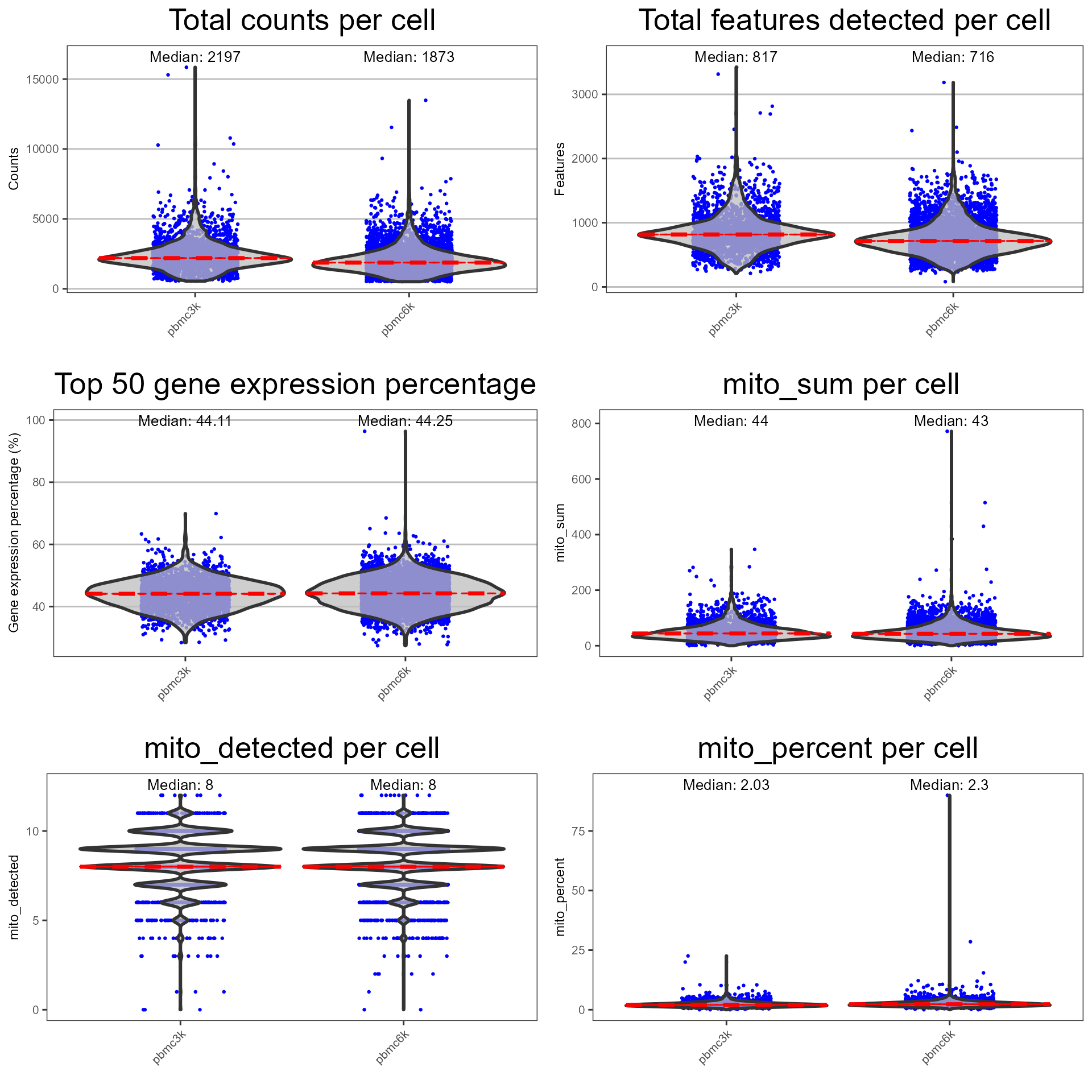
Doublet Detection
Scrublet
The wrapper function plotScrubletResults() can be used
to plot the results from the Scrublet algorithm. Here, we will use the
UMAP coordinates generated from getUMAP() in previous
sections.
reducedDims(pbmc.combined)## List of length 8
## names(8): UMAP scrublet_TSNE ... SoupX_UMAP_pbmc3k SoupX_UMAP_pbmc6k
scrublet.results <- plotScrubletResults(
  inSCE = pbmc.combined,
  reducedDimName = "UMAP",
  sample = colData(pbmc.combined)$sample,
  combinePlot = "all",
  titleSize = 10,
  axisLabelSize = 8,
  axisSize = 10,
  legendSize = 10,
  legendTitleSize = 10
)
scrublet.results 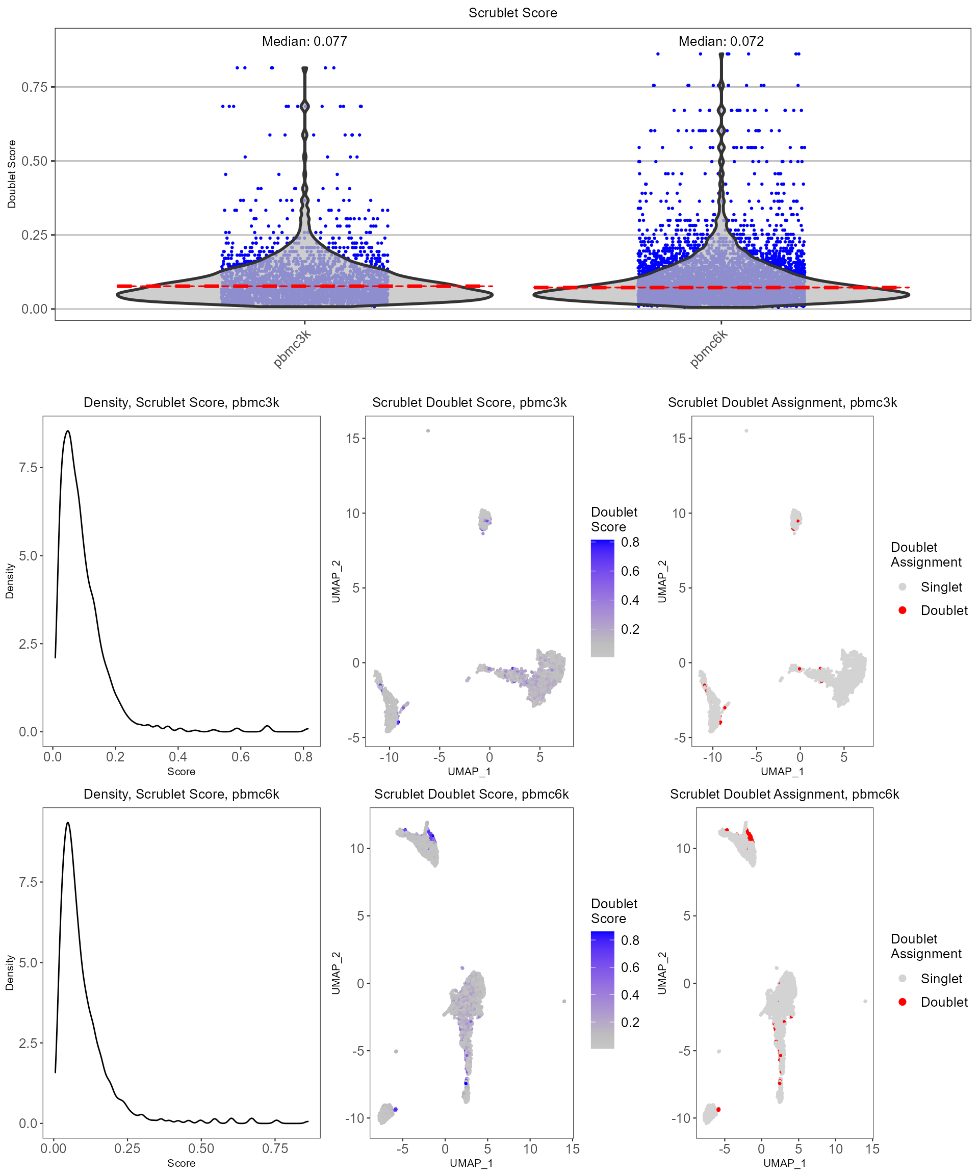
ScDblFinder
The wrapper function plotScDblFinderResults() can be
used to plot the QC outputs from the ScDblFinder algorithm.
scDblFinder.results <- plotScDblFinderResults(
  inSCE = pbmc.combined, sample = colData(pbmc.combined)$sample,
  reducedDimName = "UMAP", combinePlot = "all",
  titleSize = 13,
  axisLabelSize = 13,
  axisSize = 13,
  legendSize = 13,
  legendTitleSize = 13
)
DoubletFinder
The wrapper function plotDoubletFinderResults() can be
used to plot the QC outputs from the DoubletFinder algorithm.
doubletFinderResults <- plotDoubletFinderResults(
  inSCE = pbmc.combined,
  sample = colData(pbmc.combined)$sample,
  reducedDimName = "UMAP",
  combinePlot = "all",
  titleSize = 13,
  axisLabelSize = 13,
  axisSize = 13,
  legendSize = 13,
  legendTitleSize = 13
)
SCDS, CXDS
The wrapper function plotCxdsResults() can be used to
plot the QC outputs from the CXDS algorithm.
cxdsResults <- plotCxdsResults(
  inSCE = pbmc.combined,
  sample = colData(pbmc.combined)$sample,
  reducedDimName = "UMAP", combinePlot = "all",
  titleSize = 13,
  axisLabelSize = 13,
  axisSize = 13,
  legendSize = 13,
  legendTitleSize = 13
)
SCDS, BCDS
The wrapper function plotBcdsResults() can be used to
plot the QC outputs from the BCDS algorithm
bcdsResults <- plotBcdsResults(
  inSCE = pbmc.combined,
  sample = colData(pbmc.combined)$sample,
  reducedDimName = "UMAP", combinePlot = "all",
  titleSize = 13,
  axisLabelSize = 13,
  axisSize = 13,
  legendSize = 13,
  legendTitleSize = 13
)
SCDS, CXDS-BCDS hybrid
The wrapper function plotScdsHybridResults() can be used
to plot the QC outputs from the CXDS-BCDS hybrid algorithm.
bcdsCxdsHybridResults <- plotScdsHybridResults(
  inSCE = pbmc.combined, sample = colData(pbmc.combined)$sample,
  reducedDimName = "UMAP", combinePlot = "all",
  titleSize = 13,
  axisLabelSize = 13,
  axisSize = 13,
  legendSize = 13,
  legendTitleSize = 13
)
Ambient RNA Detection
DecontX
The wrapper function plotDecontXResults() can be used to
plot the QC outputs from the DecontX algorithm.
decontxResults <- plotDecontXResults(
  inSCE = pbmc.combined, sample = colData(pbmc.combined)$sample,
  reducedDimName = "UMAP", combinePlot = "all",
  titleSize = 8,
  axisLabelSize = 8,
  axisSize = 10,
  legendSize = 5,
  legendTitleSize = 7,
  relWidths = c(0.5, 1, 1),
  sampleRelWidths = c(0.5, 1, 1),
  labelSamples = TRUE,
  labelClusters = FALSE
)
decontxResults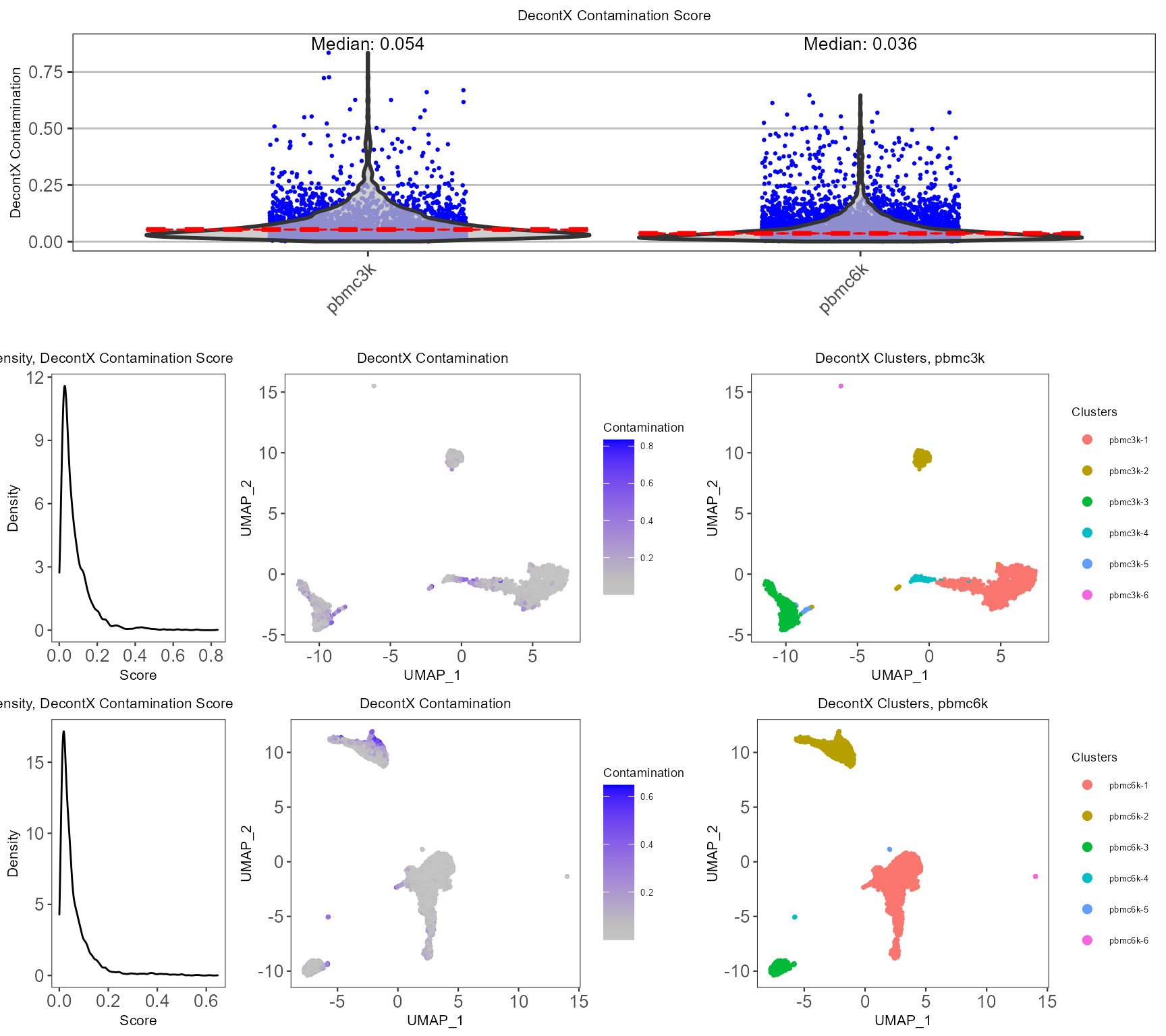
SoupX
The wrapper function plotSoupXResults() can be used to
plot the QC outputs from the SoupX algorithm.
soupxResults <- plotSoupXResults(
  inSCE = pbmc.combined, sample = colData(pbmc.combined)$sample,
  reducedDimName = "UMAP", combinePlot = "all",
  titleSize = 8,
  axisLabelSize = 8,
  axisSize = 10,
  legendSize = 5,
  legendTitleSize = 7,
  labelClusters = FALSE
)
soupxResults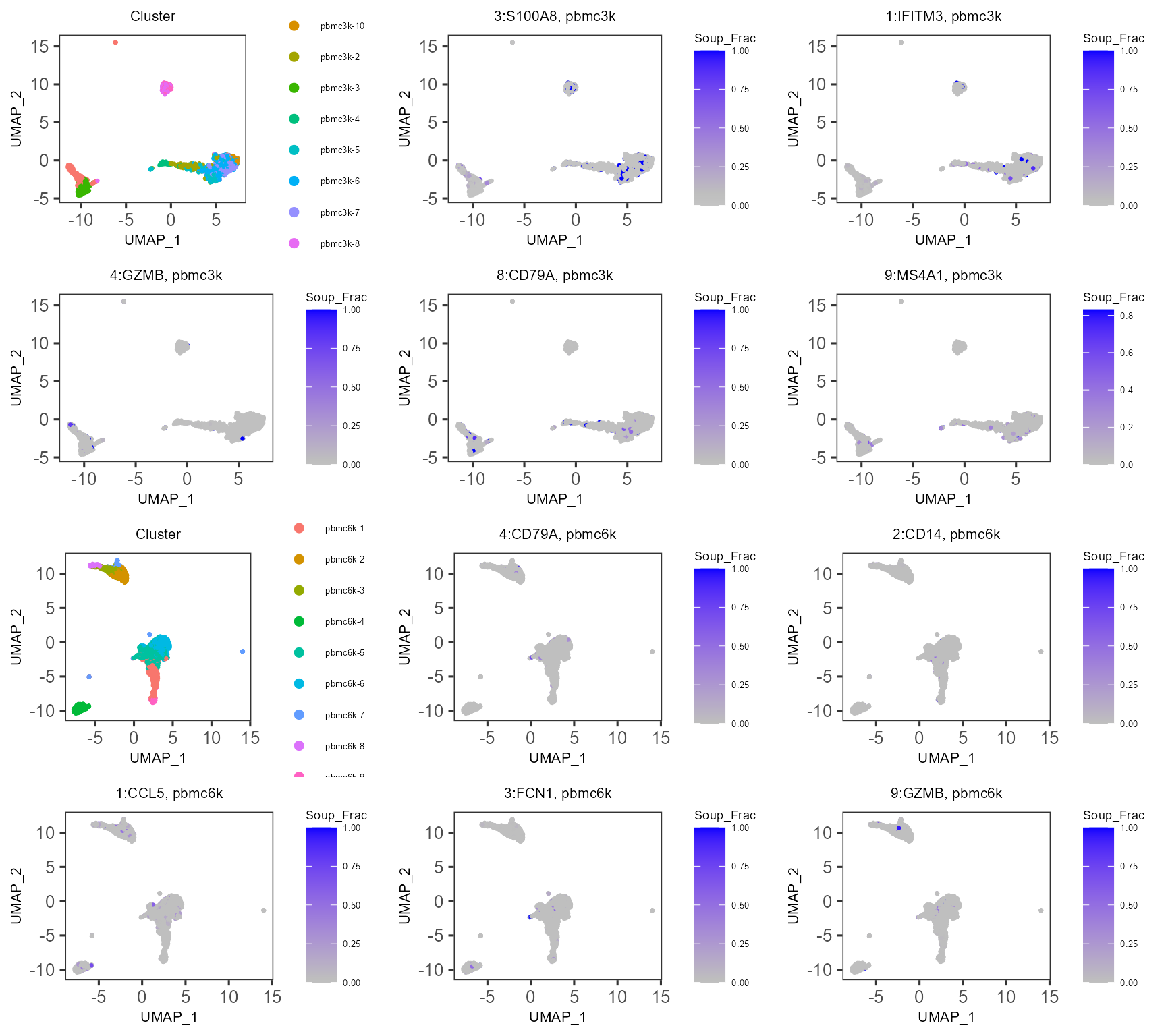
Filtering the dataset
SingleCellExperiment objects can be subset by its
colData using subsetSCECols(). The
colData parameter takes in a character vector of
expression(s) which will be used to identify a subset of cells using
variables found in the colData of the
SingleCellExperiment object. For example, if x
is a numeric vector in colData, then setting
colData = "x < 5" will return a
SingleCellExperiment object where all columns (cells) meet
the condition that x is less than 5. The index
parameter takes in a numeric vector of indices which should be kept,
while bool takes in a logical vector of TRUE
or FALSE which should be of the same length as the number
of columns (cells) in the SingleCellExperiment object.
Please refer to our Filtering
documentation for detail.
#Before filtering:
dim(pbmc.combined)
## [1] 32738 8119Remove barcodes with high mitochondrial gene expression:
pbmc.combined <- subsetSCECols(pbmc.combined, colData = 'mito_percent < 20')Remove detected doublets from Scrublet:
pbmc.combined <- subsetSCECols(pbmc.combined, colData = 'scrublet_call == "Singlet"')Remove cells with high levels of ambient RNA contamination:
pbmc.combined <- subsetSCECols(pbmc.combined, colData = 'decontX_contamination < 0.5')
#After filtering:
dim(pbmc.combined)
## [1] 32738 7931For performing QC on droplet-level raw count matrix with SCTK, please refer to our Droplet QC documentation.
Session Information
## R version 4.2.0 (2022-04-22 ucrt)
## Platform: x86_64-w64-mingw32/x64 (64-bit)
## Running under: Windows 10 x64 (build 19043)
##
## Matrix products: default
##
## locale:
## [1] LC_COLLATE=Chinese (Simplified)_China.utf8
## [2] LC_CTYPE=Chinese (Simplified)_China.utf8
## [3] LC_MONETARY=Chinese (Simplified)_China.utf8
## [4] LC_NUMERIC=C
## [5] LC_TIME=Chinese (Simplified)_China.utf8
##
## attached base packages:
## [1] stats4    stats     graphics  grDevices utils     datasets  methods
## [8] base
##
## other attached packages:
##  [1] TENxPBMCData_1.14.0         HDF5Array_1.24.1
##  [3] rhdf5_2.40.0                dplyr_1.0.9
##  [5] singleCellTK_2.7.1          DelayedArray_0.22.0
##  [7] Matrix_1.4-1                SingleCellExperiment_1.18.0
##  [9] SummarizedExperiment_1.26.1 Biobase_2.56.0
## [11] GenomicRanges_1.48.0        GenomeInfoDb_1.32.2
## [13] IRanges_2.30.0              S4Vectors_0.34.0
## [15] BiocGenerics_0.42.0         MatrixGenerics_1.8.0
## [17] matrixStats_0.62.0
##
## loaded via a namespace (and not attached):
##   [1] rsvd_1.0.5                    svglite_2.1.0
##   [3] ica_1.0-2                     assertive.properties_0.0-5
##   [5] Rsamtools_2.12.0              foreach_1.5.2
##   [7] lmtest_0.9-40                 rprojroot_2.0.3
##   [9] crayon_1.5.1                  spatstat.core_2.4-4
##  [11] MASS_7.3-57                   rhdf5filters_1.8.0
##  [13] nlme_3.1-157                  rlang_1.0.2
##  [15] XVector_0.36.0                ROCR_1.0-11
##  [17] irlba_2.3.5                   SoupX_1.6.1
##  [19] limma_3.52.2                  scater_1.24.0
##  [21] filelock_1.0.2                xgboost_1.6.0.1
##  [23] BiocParallel_1.30.3           rjson_0.2.21
##  [25] bit64_4.0.5                   glue_1.6.2
##  [27] scDblFinder_1.10.0            sctransform_0.3.3
##  [29] parallel_4.2.0                vipor_0.4.5
##  [31] spatstat.sparse_2.1-1         AnnotationDbi_1.58.0
##  [33] dotCall64_1.0-1               spatstat.geom_2.4-0
##  [35] tidyselect_1.1.2              SeuratObject_4.1.0
##  [37] fitdistrplus_1.1-8            XML_3.99-0.10
##  [39] tidyr_1.2.0                   assertive.types_0.0-3
##  [41] zoo_1.8-10                    GenomicAlignments_1.32.0
##  [43] xtable_1.8-4                  magrittr_2.0.3
##  [45] evaluate_0.15                 ggplot2_3.3.6
##  [47] scuttle_1.6.2                 cli_3.3.0
##  [49] zlibbioc_1.42.0               dbscan_1.1-10
##  [51] rstudioapi_0.13               miniUI_0.1.1.1
##  [53] sp_1.5-0                      bslib_0.3.1
##  [55] rpart_4.1.16                  RcppEigen_0.3.3.9.2
##  [57] maps_3.4.0                    fields_13.3
##  [59] shiny_1.7.1                   BiocSingular_1.12.0
##  [61] xfun_0.31                     cluster_2.1.3
##  [63] KEGGREST_1.36.2               tibble_3.1.7
##  [65] interactiveDisplayBase_1.34.0 ggrepel_0.9.1
##  [67] celda_1.12.0                  listenv_0.8.0
##  [69] Biostrings_2.64.0             png_0.1-7
##  [71] future_1.26.1                 withr_2.5.0
##  [73] bitops_1.0-7                  plyr_1.8.7
##  [75] assertive.base_0.0-9          GSEABase_1.58.0
##  [77] dqrng_0.3.0                   pROC_1.18.0
##  [79] pillar_1.7.0                  cachem_1.0.6
##  [81] fs_1.5.2                      DelayedMatrixStats_1.18.0
##  [83] vctrs_0.4.1                   ellipsis_0.3.2
##  [85] generics_0.1.2                tools_4.2.0
##  [87] beeswarm_0.4.0                munsell_0.5.0
##  [89] fastmap_1.1.0                 compiler_4.2.0
##  [91] abind_1.4-5                   httpuv_1.6.5
##  [93] rtracklayer_1.56.0            ExperimentHub_2.4.0
##  [95] plotly_4.10.0                 rgeos_0.5-9
##  [97] GenomeInfoDbData_1.2.8        gridExtra_2.3
##  [99] enrichR_3.0                   edgeR_3.38.1
## [101] lattice_0.20-45               deldir_1.0-6
## [103] utf8_1.2.2                    later_1.3.0
## [105] BiocFileCache_2.4.0           jsonlite_1.8.0
## [107] multipanelfigure_2.1.2        scales_1.2.0
## [109] graph_1.74.0                  ScaledMatrix_1.4.0
## [111] pbapply_1.5-0                 sparseMatrixStats_1.8.0
## [113] lazyeval_0.2.2                promises_1.2.0.1
## [115] doParallel_1.0.17             R.utils_2.11.0
## [117] goftest_1.2-3                 spatstat.utils_2.3-1
## [119] reticulate_1.25               rmarkdown_2.14
## [121] pkgdown_2.0.5                 cowplot_1.1.1
## [123] textshaping_0.3.6             webshot_0.5.3
## [125] statmod_1.4.36                Rtsne_0.16
## [127] uwot_0.1.11                   igraph_1.3.2
## [129] survival_3.3-1                yaml_2.3.5
## [131] systemfonts_1.0.4             htmltools_0.5.2
## [133] memoise_2.0.1                 BiocIO_1.6.0
## [135] Seurat_4.1.1                  locfit_1.5-9.5
## [137] here_1.0.1                    viridisLite_0.4.0
## [139] digest_0.6.29                 assertthat_0.2.1
## [141] mime_0.12                     rappdirs_0.3.3
## [143] spam_2.8-0                    RSQLite_2.2.14
## [145] future.apply_1.9.0            data.table_1.14.2
## [147] blob_1.2.3                    R.oo_1.25.0
## [149] ragg_1.2.2                    labeling_0.4.2
## [151] splines_4.2.0                 Rhdf5lib_1.18.2
## [153] AnnotationHub_3.4.0           RCurl_1.98-1.7
## [155] assertive.numbers_0.0-2       colorspace_2.0-3
## [157] DropletUtils_1.16.0           BiocManager_1.30.18
## [159] ggbeeswarm_0.6.0              assertive.files_0.0-2
## [161] sass_0.4.1                    Rcpp_1.0.8.3
## [163] RANN_2.6.1                    fansi_1.0.3
## [165] parallelly_1.32.0             R6_2.5.1
## [167] grid_4.2.0                    ggridges_0.5.3
## [169] lifecycle_1.0.1               bluster_1.6.0
## [171] curl_4.3.2                    leiden_0.4.2
## [173] jquerylib_0.1.4               svMisc_1.2.3
## [175] desc_1.4.1                    RcppAnnoy_0.0.19
## [177] GSVAdata_1.32.0               RColorBrewer_1.1-3
## [179] iterators_1.0.14              stringr_1.4.0
## [181] htmlwidgets_1.5.4             beachmat_2.12.0
## [183] polyclip_1.10-0               purrr_0.3.4
## [185] gridGraphics_0.5-1            rvest_1.0.2
## [187] mgcv_1.8-40                   globals_0.15.0
## [189] fishpond_2.2.0                patchwork_1.1.1
## [191] spatstat.random_2.2-0         scds_1.12.0
## [193] progressr_0.10.1              codetools_0.2-18
## [195] FNN_1.1.3.1                   metapod_1.4.0
## [197] gtools_3.9.2.2                dbplyr_2.2.0
## [199] MCMCprecision_0.4.0           RSpectra_0.16-1
## [201] R.methodsS3_1.8.2             gtable_0.3.0
## [203] DBI_1.1.3                     highr_0.9
## [205] tensor_1.5                    httr_1.4.3
## [207] KernSmooth_2.23-20            stringi_1.7.6
## [209] farver_2.1.0                  reshape2_1.4.4
## [211] annotate_1.74.0               viridis_0.6.2
## [213] magick_2.7.3                  xml2_1.3.3
## [215] combinat_0.0-8                kableExtra_1.3.4
## [217] BiocNeighbors_1.14.0          restfulr_0.0.15
## [219] scattermore_0.8               BiocVersion_3.15.2
## [221] scran_1.24.0                  bit_4.0.4
## [223] spatstat.data_2.2-0           pkgconfig_2.0.3
## [225] knitr_1.39