Version 1.1

Authors: Joshua Campbell, Rui Hong, Aaron Chevalier, Salam Alabdullatif, Christopher Husted, Yusuke Koga, Yuan Yin, Kelly Geyer
Date: 5/4/2022

1. Introduction

When developing an R package, the process of adding code that is error free, does the thing that you want it to do, and is maintainable in the long run by other users can be quite cumbersome. Several online tutorials and handbooks are available that cover various aspects of the code development process. However, a developer first needs to know what the major steps are before they can find the right resource. For example, if someone did not know about unit tests and their importance, they wouldn’t know to Google “unit test examples”.  This article provides a broad overview of the major steps that are used by the Campbell lab to add code to an existing R package. It also contains links to other articles or tutorials for many of the steps that go into more detail. Topics not included here but are worth understanding if you are an R developer include the general structure of a package, setting up a new R package, and how to write efficient R code. Additionally, this article uses GitHub for the code repository but only covers some of the basic commands. Reviewing Git tutorials is also recommended. Lastly, some of the steps listed here are optional or may vary depending on the needs of the package or development group. Overall, we hope this article will help new R developers get up to speed more quickly. If you would like to make suggestions or additional tips for this article, please email Joshua Campbell or tweet us @camplab1.

2. Install prerequisites

Several tools and R packages are used at different steps along the way. It is easiest to install all of these programs and dependencies at once.

1. Latest version of R
2. Install RStudio – RStudio is an integrated development environment (IDE) which helps developers write R code more quickly and efficiently. Most of the screenshots in this article are taken from RStudio.
3. Once you have both R and RStudio, you can install several packages that will be utilized in this tutorial:
   1. devtools – A popular to for development in R
   2. roxygen2 – For easy documentation of functions in R packages
   3. testhat – Perform unit testing in R
   4. renv – For package version management in R
   5. styler – Applies tidyverse style to code.
   6. lintr – Analyze source code for formatting and to stylistic errors
   7. usethis – Package for setting up a new package/project
   8. pkgdown – Makes a website for your R package

All packages can be installed with the following command:

install.packages(c("devtools", "roxygen2", "testhat", "renv", "styler", "lintr", "usethis", "pkgdown"))

3. Environment setup

A. Git repository

I. Fork the repo from GitHub

For this walkthrough, we will use the DevelExample repository in the campbio organization as an example. Navigate to this page and click on “Fork” in the top right corner to create a copy of the repo on your own GitHub account:

Click “Create” and then a fork will be created for your GitHub account under this link:
https://github.com/[username]/DevelExample

II. Clone the fork to your local machine

Copy the link for the repo from your GitHub page by clicking the green Code button in the top right and then copy the link:

Open your command line on your local system and navigate to the directory where you wish to store the code. Then clone the package by pasting the link after git clone :

git clone https://github.com/joshua-d-campbell/DevelExample.git

Note: If you are using a Windows system, you can use Git Bash to complete git clone and other Git related operations. Git Bash is installed when Git is installed to your Windows system.

III. Setup the remote repositories

You may eventually want to be able to get new changes that others have made to the upstream repo from the original GitHub user or organization. To do this, you need to use the “git remote” command to make a link. Go back to the GitHub page of the original repo where you forked from (“campbio” in this example). Click on the green “Clone” button and copy the text in the same way you did when you were cloning your own fork to your local machine. Go into the directory of the clone on your local machine and run git remote add [name_of_upstream] <url>  to set up the link to the upstream repo:

cd DevelExample

git remote add campbio https://github.com/campbio/devel_example.git

Some people just like to call the original repo “upstream” while others like to name it according to the name of the upstream group/user. You can then run git remote -v to view the list of remotes and double check that everything is set up correctly. You should see origin set to your own personal GitHub account and the new remote should be set to the original upstream repo which is campbio in this example.

If your R package is in Bioconductor, you may also want to set up the Bioconductor remote:

git remote add bioc git@git.bioconductor.org:packages/celda.git

Note: You will not be able to push to the Bioconductor repo unless you have permission as a maintainer. For more information on getting permission and working with Bioconductor packages, see the Bioconductor developer guide.

B. Rstudio

There are many reasons to do your coding inside Rstudio. It has integrated features for package development such as buttons for the building and checking, an IDE for highlighting R code syntax, and enhanced abilities for debugging such as adding breakpoints. The steps to create an Rstudio project to work with your package are outlined below:

1. Open Rstudio and Click New Project in the project tab on the top right part of the window:

2. If you are developing a package and already initiated a git directory for the package, choose Existing Directory:

4. Then pick the git directory of the package:

5. After clicking ‘Create Project’, Rstudio will create a new R session. Since you are in a R package folder, new options will be in the top right such as Build and Git.
6. Now you have created a new project in Rstudio which is linked the git directory of your package. Every time you make changes, you can use the Install and Restart button under the Build tab to install the current version to your library. You can also select Load All under the More button to load the current version into memory without actually installing it into your library.

4. To use the roxygen2 package to help with function documentation, click the Build item in the menu at the top of the window and then click “Configure Build Tools…”

Click Generate documentation with Roxygen in the new window. Click  “Configure…” and make sure all of the same options are checked after:

C. Manage dependencies

One challenge of contributing code to multiple packages or performing analysis on different datasets at same time is managing different versions of R package dependencies. If you rely on one particular version of a dependency for one project, but need to use newer or older versions in another project, it can be frustrating to continually install or re-install these different versions. One option to manage dependencies is by using the package renv, which allows for packages to be installed in a local folder. A brief introduction on how to setup and use local renv libraries is shown below. Although useful to create snapshots of package versions that work, this step is largely optional.

I. Set up new renv library

1. Install renv and set up a new local library:

install.packages("renv")

renv::init(bare = TRUE) # Need to restart R after this command

install.packages("BiocManager")

2. Set the global repos option to include packages from Bioconductor as well as CRAN.

options("repos" = BiocManager::repositories(version = "3.10"))

Use “version = 3.10” for R-3.6, “version = 3.11” for R 4.0, etc., according to Bioconductor release descriptions.
3. Install all package dependencies listed in DESCRIPTION file. If you have any of these already installed in your global R library, they will be linked. Otherwise, it will install the packages into the local library folder ‘renv/lib’ within your package:

renv::install()

4. Create “renv.lock” file which contains package versions. If any new dependencies are added during development, then the “snapshot” command should be run again to create a new “renv.lock” file.

renv::snapshot()

5.  Add these lines to the .gitignore file so GitHub does not keep track of the local libraries:

.Rprofile

renv/

6. Add this line to .Rbuildignore file so R does not think they are package-related files:

renv*

II. Install from existing renv

If a lock file has already been generated and is present in the repo, then you can run these commands to install versions of packages known to already work with the current version of the package:

renv::init(bare = TRUE)

renv::restore(“renv.lock”)

where “renv.lock” is the name of the appropriate lock file.

4. Adding Code

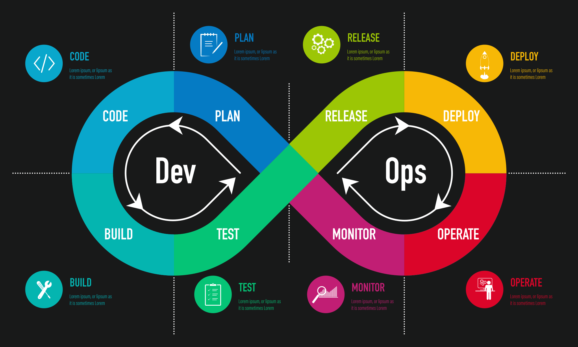
The Software Lifecycle or the systems development life cycle (SDLC) refers to the complete processes of designing, implementing, and maintaining code for a software package. Similarly, DevOps refers to  a set of practices that combines software development (Dev) and IT operations (Ops). DevOps aims to shorten the systems development life cycle and provide continuous deliverywith high software quality. Here is a nice summary of the steps that can be involved in DevOps:
 
In this section, we will only focus on the “Dev” side related to coding, building, and testing R packages with GitHub.

A. Before adding code

I. Choose the appropriate branch

Understanding how the particular repo you are working with uses different branches for different purposes is important so you can know where and when to add your code. Different organizations and repos may have different practices so you will need to look at their documentation or ask their developers. For example, one group might just use “master” or “main” as the primary branch and everyone can push/pull code from directly to/from it all the time. In this tutorial, we make use of both a “devel” and a “master” branch. Developers push changes to the “devel” branch when making updates. Only stable versions are pushed to the “master” branch along with a version bump and corresponding new release. For our DevelExample repo, run this command to switch to the “devel” branch if not already there:

git checkout devel

Or you can do this within Rstudio by clicking on Git tab in the top right and selected devel from the drop down box:

Note: You may also want to create your own separate branch from devel if you are making substantial changes. This can be done with the command git checkout -b <new_branch_name>. See this article for more information on utilizing Git branches.  

II. Merge/Pull changes from upstream repos

If you just cloned the repo, then chances are that you have the latest version of the code and do not need to worry about syncing with the upstream repo. If you have been working on a package for a while along with other developers, then your local version of the package may be behind the upstream repo in the original organization (”campbio” in this example). It is often a good idea to incorporate changes that other developers have made before starting to add or change code on your local repo as this may help reduce potential merge conflicts later on. Here is the code to fetch the latest code:

git fetch campbio

git merge campbio/devel

Similar functionality can be done with git pull. See this article for more information on Git fetching/pulling and comparisons between them. If you have already started making changes to your local repo and then try to merge from an upstream repo, you may already have merge conflicts. These can be resolved with git mergetool or with other text editors.  See this article for a brief introduction to merging in Git or Google “Git merge conflicts” to find any number of tutorials/examples.

B. Adding code to the package

If you are starting a package from scratch, you can read through other tutorials about how to set up the package structure, including ones from Hadley Wickham or Fong Chun Chan. However, this only needs to be done once. So most of the time, you will be adding code to an existing package.

I. Function code

Most of the code in your R package will be enclosed within an R function. In this tutorial, we will add a function to the DevelExample package that calculates the Euclidean distance between two vectors. Below is an example of an R function that calculates this distance and another one that checks for NAs in our vectors. This code can be copied into a new file called “distance.R” in the R directory of the package.

euclideanDist <- function(a, b, verbose = FALSE) {
  if (isTRUE(verbose)) {
    message("Calculating distance ...")
  }

  # Check validity of data
  .check_data_integrity(a)
  .check_data_integrity(b)

  # Perform calculation
  res <- sqrt(sum((a-b)^2))
  return(res)
}

.check_data <- function(input) {
  if (any(is.na(input))) {
    stop("'input' must not contain NAs")
  }
}

To test your function, you can run the command devtoools::load_all() which will load the current version of your code into the R environment without actually reinstalling the package. You can also run this by selecting Load All after clicking More under the Build tab in Rstudio:

In this example, we actually put some of the code inside of a “dot” utility function (i.e. the function starting with a “.”). There are two reasons to split up code for your function into smaller functions. The first reason is if that chunk of code will be used or called in multiple places or from multiple functions across your package. It is generally a bad idea to have redundant code in multiple places as it is harder to maintain when changes to the code will inevitably be needed in the future. The second reason is if your function is long because it contains multiple, complex parts. If your function can be split up into smaller steps with each step coded in its own small function, this will improve the design, maintainability, and readability of the overall function. Note that these functions do not actually have to start with a period, but it is a convention that some groups like to use to help developers distinguish between the functions that they want users to see versus internal functions they use to better organize the code (i.e. exported vs non-exported functions).
Here is a brief list of some additional best practices to make your code consistent and maintainable:

• Standard function naming. If you are adding to an existing repo, make sure to understand the conventions for that repo. Make sure to use standard conventions for function and parameter names. Common naming conventions include camel case (e.g. euclideanDist), snake case (e.g. euclidean_dist), or Google’s R style guide (e.g. EuclideanDist). Understand if there are preferences for abbreviated words or full words in function names (eucl_dist vs. euclidean_distance). It is also a good idea to document these preferences in a developer wiki.
• File organization and naming. If you have a lot of functions, it is generally a good idea to split them up in multiple files. Multiple functions should only be in the same file if they are functionally related. Many packages keep separate files for the accessors and utility functions. It is also a good idea to think through the convention for the names of these files so other developers can quickly find the code they want to understand or modify.
• Namespace. Always remember to specify the namespace of each function from other packages in case other package has a function (e.g. stats::anova instead of anova). You can also use import to import several functions at a time. When you build and check the package later, you will get warnings if you do not call functions properly. See this chapter on namespaces for more information.
• Accessor functions. These types of functions are a staple of programming (OOP). Do not directly use “@” to access slots in an S4 object. Use the package-specified accessor functions. For example, do not use obj@metadata to access the metadata from an object, but use metadata(sce). This is because the locations of data may change within the object in new releases, but the accessor functions should be more static and always return the same underlying data. See this article on S4 objects for more info.
• Boolean flags. Use TRUE and FALSE and not T or F. T/F are just variable set to TRUE/FALSE that can be changed. When checking Boolean flags in “if” statements, use the isTRUE() function like this if(isTRUE(flag)) {…} . For example if(1) will be evaluated as TRUE and run whereas if(isTRUE(1)) will be evaluated as FALSE and not run.

II. Function documentation

Each function should be fully documented including title, description, parameters, return, and examples. This may also include additional sections for details and “see also”. Read the tutorials from the R packages book and roxygen2 vignette for a more complete description of the different documentation elements with examples. Here are our functions that calculate Euclidean distance with documentation added:

#' @title Euclidean distance
#' @description Calculates Euclidean distance between two vectors. An error will be
#' given if NAs are present in either vector.
#'
#' @param a The first vector to use in the distance calculation.
#' @param b The second vector to use in the distance calculation.
#' @param verbose Boolean. If \code{TRUE}, a message will be printed. Default \code{TRUE}.
#' @return A numeric value of a distance
#' @examples
#' euclideanDist(c(1, 2), c(2, 3), verbose = FALSE)
#' @export
euclideanDist <- function(a, b, verbose = FALSE) {
  if (isTRUE(verbose)) {
    message("Calculating distance ...")
  }

  # Check validity of data
  .check_data(a)
  .check_data(b)

  # Perform calculation
  res <- sqrt(sum((a-b)^2))
  return(res)
}

.check_data <- function(input) {
  if (any(is.na(input))) {
    stop("'input' must not contain NAs")
  }
}

One the function documentation has been written, you can run devtools::document() to write/update man .Rd files and the NAMESPACE file. You can also use the shortcut Shift + Ctrl/Cmd + d or select Document after clicking More under the Build tab in Rstudio:

Remember that only functions with the @export tag will be visible to the user. You can preview documentation with ?functionName  (?euclideanDist in this example) and then make modifications as needed.

III. Example data

Many function examples will need to run on some sort of data. Sometimes it is more efficient to save a small dataset within the R package, especially if it can be used as the input for several examples. R packages have the ability to to include data in a few different ways which are described in the External data chapter of the R Packages book. We will use the first way of storing example data using the data/ folder. First we run the following code to set up the data-raw folder (if it has not been set up already):

usethis::use_data_raw(name = "example_data")

This will also create a file in data-raw folder called example_data.R which we can use to store code that creates the example dataset. Note that this folder is added to the .Rbuildignore file so it (and all of the files within it) will be included in our GitHub repo but not in the bundled version of the package.
Here is the code we put in the file and then run to create and save an example dataset with two vectors:

## code to prepare `example_data` dataset goes here
set.seed(123)
a <- rnorm(100)
b <- rnorm(100)
example_data <- cbind(a, b)
usethis::use_data(example_data, overwrite = TRUE)

All data objects must also be documented. In order to document this example dataset, we can create a file called data.R in the R subdirectory with the following code:

#' Example dataset
#'
#' A dataset containing a matrix with two columns that were generated
#' with a random normal distribution with a mean of 0 and stdev of 1. 
#'
#' @format A matrix with 100 rows and 2 columns
#' @keywords datasets
#' @usage data("example_data")
#' @examples
#' data("example_data")
"example_data"

Also include and @source tag if you returned the data from an outside database or website.

We can now update the original @examples code in our function euclideanDist to use this example dataset instead:

#' @examples
#' data(example_data)
#' euclideanDist(example_data[,1], example_data[,2], verbose = FALSE)

Make sure to rerun devtools::document() to generate the man file for the example datasets and update the function documentation.

IV. Committing code

As we are working with Git, we will need to continually commit the new code to the repo at some point. It is generally up to the developer how often they commit changes. Commits can be made after each small addition (e.g. separate commits for the main function code, documentation, example data, unit tests, etc.) or after major blocks of updates have been made (e.g. one major commit for all of the main function code, documentation, example data, unit tests, etc.). Here, we will demonstrate a commit for the last step of adding the example dataset. Here is the git commands that can add the new files and commit the changes (assuming we are on the “devel” branch):

git add R/data.R data-raw/ data man/example_data.Rd

git commit -a -m "Added new example_dataset and used it in the example for the euclideanDist function"

Committing code can also be achieved in Rstudio. Select the Git tab and then check all of the files to be added during this next commit:

After checking all files to add/stage, select the Commit button:

Add an informative message describing all of the changes that will be included and then select Commit to add the code to the branch:

While no more commits will be explicitly shown during this tutorial, all of the remaining steps will be committed before creating the Pull Request (PR) at the end.

C. Units tests

Unit testing is a way of testing the smallest piece of code that can be logically isolated in a system. The testthat package can be used to easily set up and run unit tests in R. Unit tests may not be super useful for the code you are adding at this point as you have likely tested it in prior steps. However, they are extremely useful when making future updates to ensure that new changes do not break existing functionality across your package.

I. Initial setup.

To set up testthat, you can run usethis::use_testthat() . This will create a tests/testthat directory, add “testthat” to the Suggests field in the DESCRIPTION file, and create a file called tests/testthat.R that runs all your tests. This setup step should only need to be performed one time for a package. See the testthat tutorial for more information. The unit tests for our DevelExample package were initialized with the following commands:

library(usethis)
use_testthat()
use_test()

II. Adding unit tests

Once new code has been added, we can make a series of unit tests to check the validity of the code. Test files must be put into the tests/testthat directory and start with the prefix “test”. Each file can contain a series of tests defined by the test_that function and each test can contain one or more expectations. Details about the different types of expectations can be found here.
For our example, we will create a new file called test-euclidean.R containing the following code with two unit tests:

library("DevelExample")
data(example_data)
test_that("Testing euclideanDist function", {
  res <- dist(rbind(example_data[,1], example_data[,2]))[1]
  expect_equal(euclideanDist(example_data[,1], example_data[,2]), res)

  expect_error(euclideanDist(c(1, 2), c(NA, 2)), regexp = "contain NAs")
})

The first unit test ensures that our distance calculation matches the one performed by the dist function and the second unit test ensure that our check for NAs works and throws an error. Once the unit tests are added, you can run them by pressing Ctrl/Cmd + Shift + t in Rstudio, by running devtools::test() in the R console, or by clicking More and then selecting Test Package in the Rstudio:

By changing code in one part of the package, you may break code in another part of the package. Make sure all of your unit tests pass before moving on to the next major steps, even if it is another part of the code that is breaking.

III. Checking coverage

Your can generate a coverage report to inspect coverage for each line in your package using the covr package:

library(covr)
report()

In an ideal world, your package would have 100% coverage. However, this may not be completely feasible depending on the size of the package, the number of permutations for various use cases, and speed which it takes to check all functions. Coverage reports can also be generated and reviewed with GitHub Actions when making a Pull Request.

D. Build and Check (Initial)

Checking all of your code for common problems is important to do for each new piece of code that is being added. Sometimes adding new code or changing previous can cause unintended errors or problems in other parts of the package. R CMD build and R CMD check are built-in R commands that build the package tarball and run several different tests, respectively. R CMD check runs unit tests, checks for consistency between the documentation and function parameters, checks for discrepancies in namespace and dependency usage, and much more.  We suggest doing two rounds of checking. The first round shown here will not re-build the vignettes or test examples with the \dontrun{} command. You should be able to fix the majority of new issues in this step. In a later “final” check, we will test whole the re-building of the vignettes and other functions.

I. Initial setup (Optional)

To change the default parameters for the building/checking tools in RStudio, click the Build tab in the top right, click the More option in the dropdown list, and select Configure Build tools.

Adding the —no-build-vignettes flag to the Check and Build options will speed up the process if the vignette takes a long time to run. If your vignette is fast, then you can skip this step.

II. Performing the check

When you finished editing the code, click Check in the Build window to check the package:

The checks will run in the top right panel and may return a ERROR, WARNING, or NOTE. Make sure you fix all new issues (with warnings and errors being the most important) before moving on to the next steps. You can ignore the NOTE related to files in your .git subfolder being too large or the NOTE that there are too many dependencies. In the R console, you can also just type devtools::check_man() in the console to only check the documentation or devtools::run_examples() to only check the examples. More details on R CMD check can be found here. You may also want to perform this check after each individual step listed in this tutorial.

E. Code style

I. Run styling functions

The styler R package can be used to reformat code to help ensure consistent formatting. You can run style_pkg() , style_dir() , or style_file() to style the entire package, a directory, or a file, respectively. See the documentation on the styler website for more details. This can also be run easily in Rstudio by clicking Code in the top menu and selecting Reformat Code.

II. Checking the style

The package lintr can be used to analyze the format and style of source code. It checks for adherence to a given style, syntax errors, and other possible semantic issues. You can use lint_package(), lint_dir(), or lint() to lint an entire package, directory, or file, respectively. The default of lintr is to look for “snake_case” format. To use “camelCase” format, you can give the following command:

lint_package(linters = with_defaults(object_name_linter = object_name_linter("camelCase")))

A configuration file called .lintr can be created in the top level of the R package directory. See the instructions on lintr’s GitHub page for setting up the config file and turning on/off various lints.

F. Vignettes

Vignettes are short tutorials used to showcase the functionality of your package using example data. Vignettes can be written in Rmarkdown and compiled with knitr. As the vignettes are often built and distributed with the package, they should be able to run in a relatively short period of time. Therefore using a small example or a toy dataset is usually recommended. If your workflow takes longer to run on real-world data, this can be demonstrated in separate articles with pkgdown (described later).
For this tutorial, we will add a simple chunk of code in the existing vignette file called DevelExample.Rmd that describes our new function for calculating Euclidean distance:

To calculate the euclidean distance between two vectors, we can use the `euclideanDist` function. In this example we will generate two random vectors from normal distributions with two different means and calculate the distance between them:

```{r dist}
set.seed(12345)
v1 <- rnorm(10000, mean = 1)
v2 <- rnorm(10000, mean = 2)
res <- euclideanDist(v1, v2, verbose = FALSE)
res
```

The `set.seed` function is used for the random number generator and ensures the same vectors will be produced each time for reproducibility.

G. Build and Check (Final)

After completing all style checking and vignettes, it is a good idea to do one final local check which includes re-building of all the vignettes (if not done previously) and running of all examples. Instead of changes the options in the Configure Build Tools window, you can run a more complete check in the R console with the following command:

devtools::check(document = FALSE, vignettes = TRUE, run_dont_test = TRUE)

Setting document = FALSE forces the check function to not run devtools::document(). All function documentation writing should be done in the previous steps and any errors should be captured and fixed at this stage. Setting vignettes = TRUE will make all vignettes be rebuilt and tested. The run_dont_test = TRUE will force examples tagged with \donttest{} to be run and checked for errors. These functions may not be tested elsewhere, so it is a good idea to test them at this point. You can also set the ーrun-donttest flag in the Check options under the Configure Build Tools to achieve the same behavior in Build window.

Note: Make sure this build/check does not return new warnings or errors on your local system before proceeding.

If this is a Bioconductor package, this is also a good time to perform Bioconductor specific checks on your local system. This can be done by installing the package BiocCheck and running the command BiocCheck::BiocCheck(). Make sure to address errors and warnings and minimize the number of notes as this will save some time when pushing to the official Bioconductor repository.

H. Update version

The version of the package is encoded in the DESCRIPTION file and looks like Version: 1.1.0. The three numbers correspond to MAJOR.MINOR.PATCH versions. In general, the MAJOR version should be updated when you make incompatible changes with previous version, the MINOR version should be updated when you add functionality in a backwards-compatible manner, and the PATCH version should be updated when you make backwards-compatible bug fixes. See this article for best practices when using semantic versioning. Note that Bioconductor has its own versioning system where the MINOR version is increased in the development and release branches of the Bioconductor repo. In this tutorial, we will bump the MINOR version number to 1 since this is still a pre-release of our new package:  Version: 0.1.0.

I. Update NEWS

The NEWS file describes the series of changes that have been made to your package throughout its version history. The markdown version of the NEWS file will also be displayed in the pkgdown website. To initialize this file, run the command usethis::use_news_md(). Each new version should be denoted with a # and can have a list of bullet points that summarize the changes. For this tutorial, we will add a new version and a line that describes the addition of the new euclidean distance function to the top of the NEWS.md file:

# Changes in Version 0.1.0 (2022-05-20)
* Added function to calculate euclidean distance

If you are adding changes but not yet ready to create a new release, it is still a good idea to make updates to the NEWS file right after adding new features or fixing bugs. Otherwise, you may forget what features were added later on when updating the release number. To get around this, a temporary “dummy” release can be made in the NEWS file where bullet points can be added as new updates to the package are made:

# Changes in Version X.X.X (20XX-XX-XX)
* Added function to do something important
* Fixed bugs in another function
* Reformatted vignette

When all of the relevant features and bug fixes have been finalized and it is time to cut the new release, the version number and dates can then be updated accordingly.

J. Website

The pkgdown R package can be used to build a website on top of your R package. To initialize the pkgdown structure, you can run the following commands:

usethis::use_pkgdown()

And to build the website each time, the following command can be run:

pkgdown::build_site()

By default, the vignettes will be built and made available under the “Getting started” tab in the website. However, additional tutorials coded in R markdown can be placed in subdirectories such as vignettes/articles. In contrast to the vignettes (which are supposed to be short and use small toy datasets), the articles are a good way to demonstrate full-length workflows on real-world datasets. If pkgdown has already been initialized, you may want to write and test the articles at the same time as the vignettes in the previous step. However, the site should always be rebuilt after the updates to the version number and NEWS file as this information will be displayed in the website.
Various aspects of the website can be customized by modifying the “_pkgdown.yaml” file. This website can be published with GitHub pages or put on your own website. This process can be automated with GitHub Actions as well.

Note: When adding new code or functionality, make sure to update the appropriate articles that are separate from the vignettes. This often serves as another layer of checking to ensure your new code is robust.  

K. Merge final code

I. Create a Pull Request (PR)

Creating a Pull Request is a common way to merge your changes into the upstream repo in the original organization. After you have committed all of your changes to your local devel branch, you can push this to the origin repo in your GitHub with the following code:

git push origin devel

One of the easiest way to make a PR is to navigate to your GitHub repo in a web browser and click on Pull requests:

Click on New Pull Request and then select the branches that you want to merge. In this tutorial, we will be making a PR from the devel repo in the fork (joshua-d-campbell) to the devel repo in the original organization (campbio):

Click on Create pull request and then fill in the Title and Description fields with some useful text:

Click on Create pull request when ready to submit the final PR. Optionally, you can select Reviewers on the right to assign the review process to an individual.

II. Continuous integration

GitHub Actions is a continuous integration tool for GitHub repo which ensures that your software can compiled and checked successfully in multiple environments. Multiple workflows can be setup and run in parallel. Generally, workflows only need to be set up once. The usethis  package provides a set of convenient functions to setup various workflows. For example, usethis::use_github_action_check_full() will create a workflow for R CMD Check andusethis::use_github_action(“lint”) will create a workflow for lintr. All workflow configuration yaml files are available in .github/workflows subfolder. These files can be updated to modify dependencies or make other changes to each workflow. For example, changes to the configuration files R-CMD-check.yaml may be required if a R or Python dependency was not included. In general, this step only needs to be set up once but the configuration files will sometimes will require occasional updates. Other CI tools such as travis may also be used for this purpose.
After submitting your PR, all of the GitHub Action workflows will start running:

If any of the workflows failed, click on the workflow to access the log and see what the error is:

Use the previous steps in this tutorial to fix any errors in the code and perform the standard checks. When you push your code back to your origin branch, you do NOT need to make a new PR. Your original PR will update and the GitHub Action workflows will automatically restart. Keep refining code until that all checks have passed:

III. Accept

After all GitHub workflows have passed and the code has been reviewed, the package maintainers (or you) can accept the PR and your code will be incorporated into the devel branch in the upstream repo. Congratulations! By performing all of these steps, you can take comfort in knowing that you contributed maintainable and readable code to an important repo!