Feature Selection
Irzam Sarfraz
Source:vignettes/articles/cnsl_feature_selection.Rmd
cnsl_feature_selection.RmdIntroduction
singleCellTK offers a convenient way to compute and select the most variable features that show the highest biological variability to use them in the downstream analysis. Feature selection methods available with the toolkit include vst, mean.var.plot & dispersion from Seurat [1][2][3][4] package and modelGeneVar from Scran [5] package. Users can additionally use visualization options and methods to visualize the top variable genes interactively as well as from R console.
To view detailed instructions on how to use these methods, please select ‘Interactive Analysis’ for using feature selection in shiny application or ‘Console Analysis’ for using these methods on R console from the tabs below:
Workflow Guide
1. Select Feature Selection & Dimensionality Reduction tab from the top menu. This workflow guide assumes that the data as been previously uploaded, filtered and normalized before proceeding with this tab. 
2. Select Feature Selection sub-tab (selected by default) to open up the feature selection user-interface.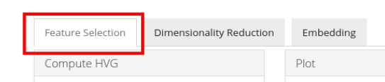
3. The Feature Selection sub-tab is divided into three panels namely, a) Compute HVG, b) Select and Subset, and c) Plot. 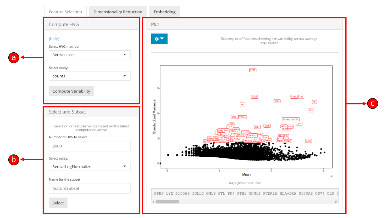
The working of sections a, b and c are described below:
a) Compute HVG
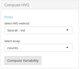
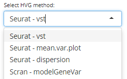
The Compute HVG window allows the processing of highly variable genes by selecting an appropriate method either from Seurat (vst, mean.var.plot, dispersion) or Scran (modelGeneVar) packages.
A numeric value indicating the number of features to identify must be set (default is 2000) and an assay must be selected from the list of available assays.
b) Select and Subset
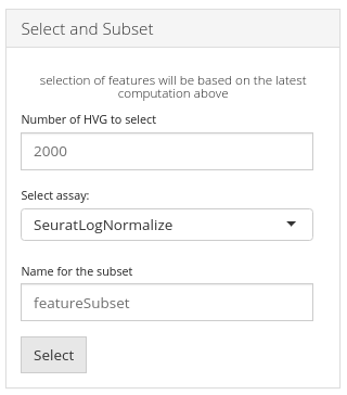
Once the highly variable genes have been computed in (a), subset of these features can be selected for downstream analysis. A numeric value (default is 100) can be input to set the number of genes that should be displayed in (b), labeled (highlighted in red) in the plot (c) and selected for further analysis in the succeeding tabs as a subset.
c) Plot
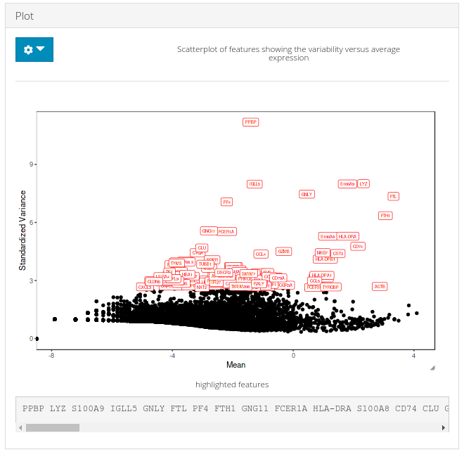
A plot is generated against the HVG computation in (a) and the number of genes to display set in (b) are labeled over corresponding data points in the plot.
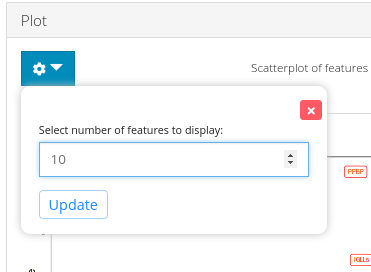
To change the number of variable genes to highlight, plot options can be opened up as shown in the figure above.
1. Compute statistics for the highly variable genes using the wrapper function runFeatureSelection as below:
sce <- runFeatureSelection(inSCE = sce, useAssay = "counts", hvgMethod = "vst")In the above function, it is recommended to use a normalized assay for the useAssay parameter and the available options for the hvgMethod method include vst (recommended assay is raw counts), mean.var.plot and dispersion from Seurat and modelGeneVar from Scran package.
2. Get names of top genes using the getTopHVG function and specify the same method which was used for computation in the step 1:
topGenes <- getTopHVG(inSCE = sce, method = "vst", n = 1000)3. Visualize top genes using the plotTopHVG function and specify the same method which was used previously:
plotTopHVG(inSCE = sce, method = "vst", hvgList = topGenes, labelsCount = 10)Example
  # Load singleCellTK & pbmc3k example data
  library(singleCellTK)
  sce <- importExampleData(dataset = "pbmc3k")
  # Compute metrics for 'vst' feature selection method
  sce <- runFeatureSelection(inSCE = sce, useAssay = "counts", hvgMethod = "vst")
  # Get the names of the top 1000 highly variable genes
  topGenes <- getTopHVG(inSCE = sce, method = "vst", n = 1000)
  print(topGenes[1:10])
## [1] "PPBP" "LYZ" "S100A9" "IGLL5" "GNLY" "FTL" "PF4" "FTH1"
## [9] "GNG11" "FCER1A"
  # Visualize the top variable genes and label the first top 10 genes
  plotTopHVG(inSCE = sce, method = "vst", hvgList = topGenes, labelsCount = 10)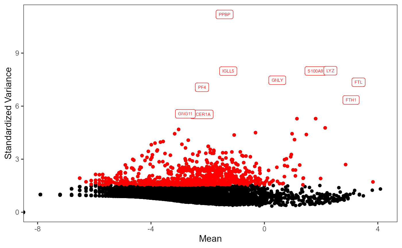
Individual Functions
While the runFeatureSelection wrapper function can be used to run all available feature selection methods, separate functions are also available for all of the included methods. The following functions can be used for specific feature selection methods:
vst, mean.var.plot or dispersion from Seurat [1][2] package:
sce <- seuratFindHVG(inSCE = sce, useAssay = "counts", hvgMethod = "vst", hvgNumber = 2000, altExp = FALSE, verbose = TRUE)The parameters to the above function include: inSCE: an input SingleCellExperiment object useAssay: specify the name of the assay to use for feature selection hvgMethod: one of the options from “vst,” “mean.var.plot” or “dispersion” hvgNumber: specify the number of variable genes to compute by default altExp: a logical value indicating if the input object is an altExperiment verbose: a logical value indicating if progress should be printed
modelGeneVar from Scran package:
sce <- scranModelGeneVar(inSCE = sce, assayName = "counts")The parameters to the above function include: inSCE: an input SingleCellExperiment object assayName: selected assay to compute variable features from