vignettes/articles/decontX_pbmc4k.Rmd
decontX_pbmc4k.RmdIntroduction
Droplet-based microfluidic devices have become widely used to perform single-cell RNA sequencing (scRNA-seq). However, ambient RNA present in the cell suspension can be aberrantly counted along with a cell’s native mRNA and result in cross-contamination of transcripts between different cell populations. DecontX is a Bayesian method to estimate and remove contamination in individual cells. DecontX assumes the observed expression of a cell is a mixture of counts from two multinomial distributions: (1) a distribution of native transcript counts from the cell’s actual population and (2) a distribution of contaminating transcript counts from all other cell populations captured in the assay. Overall, computational decontamination of single cell counts can aid in downstream clustering and visualization.
The package can be loaded using the library command.
library(celda)DecontX can take either SingleCellExperiment object from package SingleCellExperiment package or a single counts matrix as input. decontX will attempt to convert any input matrix to class dgCMatrix from package Matrix before beginning any analyses.
Load PBMC4k data from 10X
We will utlize the 10X PBMC 4K dataset as an example. This can be easily retrieved from the package TENxPBMCData. Make sure the the column names are set before running decontX.
# Install TENxPBMCData if is it not already
if (!requireNamespace("TENxPBMCData", quietly = TRUE)) {
  if (!requireNamespace("BiocManager", quietly = TRUE)) {
    install.packages("BiocManager")
  }
  BiocManager::install("TENxPBMCData")
}

# Load PBMC data
library(TENxPBMCData)
sce <- TENxPBMCData("pbmc4k")
colnames(sce) <- paste(sce$Sample, sce$Barcode, sep = "_")
rownames(sce) <- rowData(sce)$Symbol_TENx
Running decontX
A SingleCellExperiment (SCE) object or a sparse matrix containing the counts for filtered cells can be passed to decontX via the x parameter. There are two major ways to run decontX: with and without the raw/droplet matrix containing empty droplets. The raw/droplet matrix can be used to empirically estimate the distribution of ambient RNA, which is especially useful when cells that contributed to the ambient RNA are not accurately represented in the filtered count matrix containing the cells. For example, cells that were removed via flow cytometry or that were more sensitive to lysis during dissociation may have contributed to the ambient RNA but were not measured in the filtered/cell matrix. The raw/droplet matrix can be input as a sparse matrix or SCE object using the background parameter:
sce <- decontX(sce, background = raw)If cell/column names in the raw/droplet matrix are also found in the filtered counts matrix, then they will be excluded from the raw/droplet matrix before calculation of the ambient RNA distribution. If the raw matrix is not available, then decontX will estimate the contamination distribution for each cell cluster based on the profiles of the other cell clusters in the filtered dataset:
sce <- decontX(sce)Note that in this case decontX will perform heuristic clustering to quickly define major cell clusters. However if you have your own cell cluster labels, they can be specified with the z parameter. If you supply a raw matrix via the background parameter, then the z parameter will not have an effect as clustering will not be performed.
The contamination can be found in the colData(sce)$decontX_contamination and the decontaminated counts can be accessed with decontXcounts(sce). If the input object was a matrix, make sure to save the output into a variable with a different name (e.g. result). The result object will be a list with contamination in result$contamination and the decontaminated counts in result$decontXcounts.
Plotting DecontX results
Cluster labels on UMAP
DecontX creates a UMAP which we can use to plot the cluster labels automatically identified in the analysis. Note that the clustering approach used here is designed to find “broad” cell types rather than individual cell subpopulations within a cell type.
umap <- reducedDim(sce, "decontX_UMAP")
plotDimReduceCluster(x = sce$decontX_clusters,
    dim1 = umap[, 1], dim2 = umap[, 2])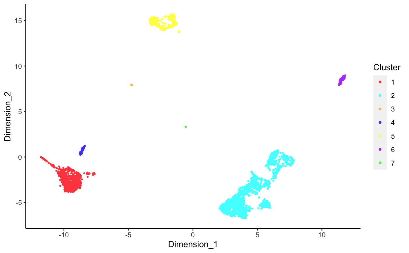
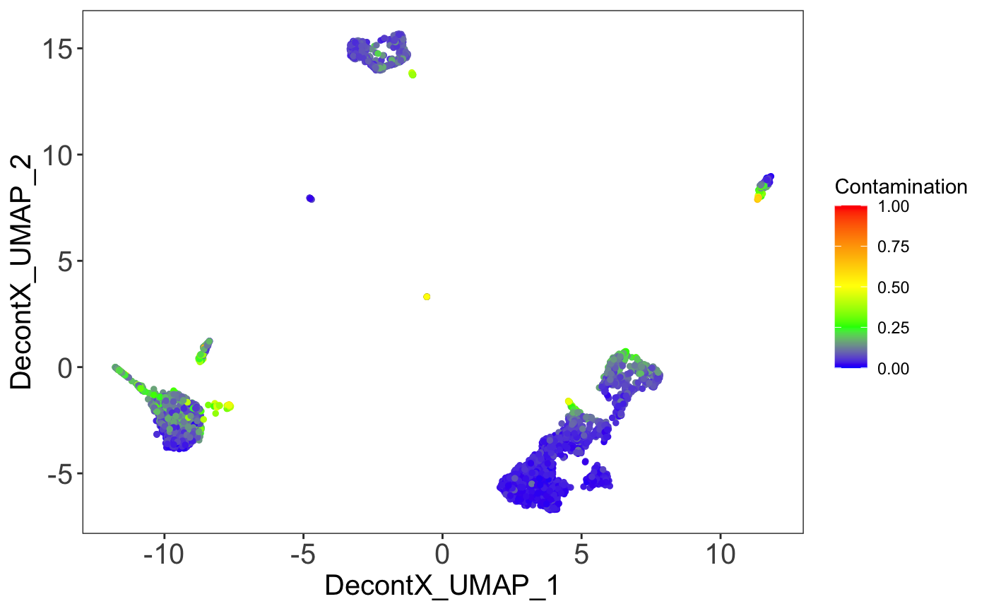
Contamination on UMAP
The percentage of contamination in each cell can be plotting on the UMAP to visualize what what clusters may have higher levels of ambient RNA.
Expression of markers on UMAP
Known marker genes can also be plotted on the UMAP to identify the cell types for each cluster. We will use CD3D and CD3E for T-cells, LYZ, S100A8, and S100A9 for monocytes, CD79A, CD79B, and MS4A1 for B-cells, GNLY for NK-cells, and PPBP for megakaryocytes.
library(scater)
sce <- logNormCounts(sce)
plotDimReduceFeature(as.matrix(logcounts(sce)),
    dim1 = umap[, 1],
    dim2 = umap[, 2],
    features = c("CD3D", "CD3E", "GNLY",
        "LYZ", "S100A8", "S100A9",
        "CD79A", "CD79B", "MS4A1"),
    exactMatch = TRUE)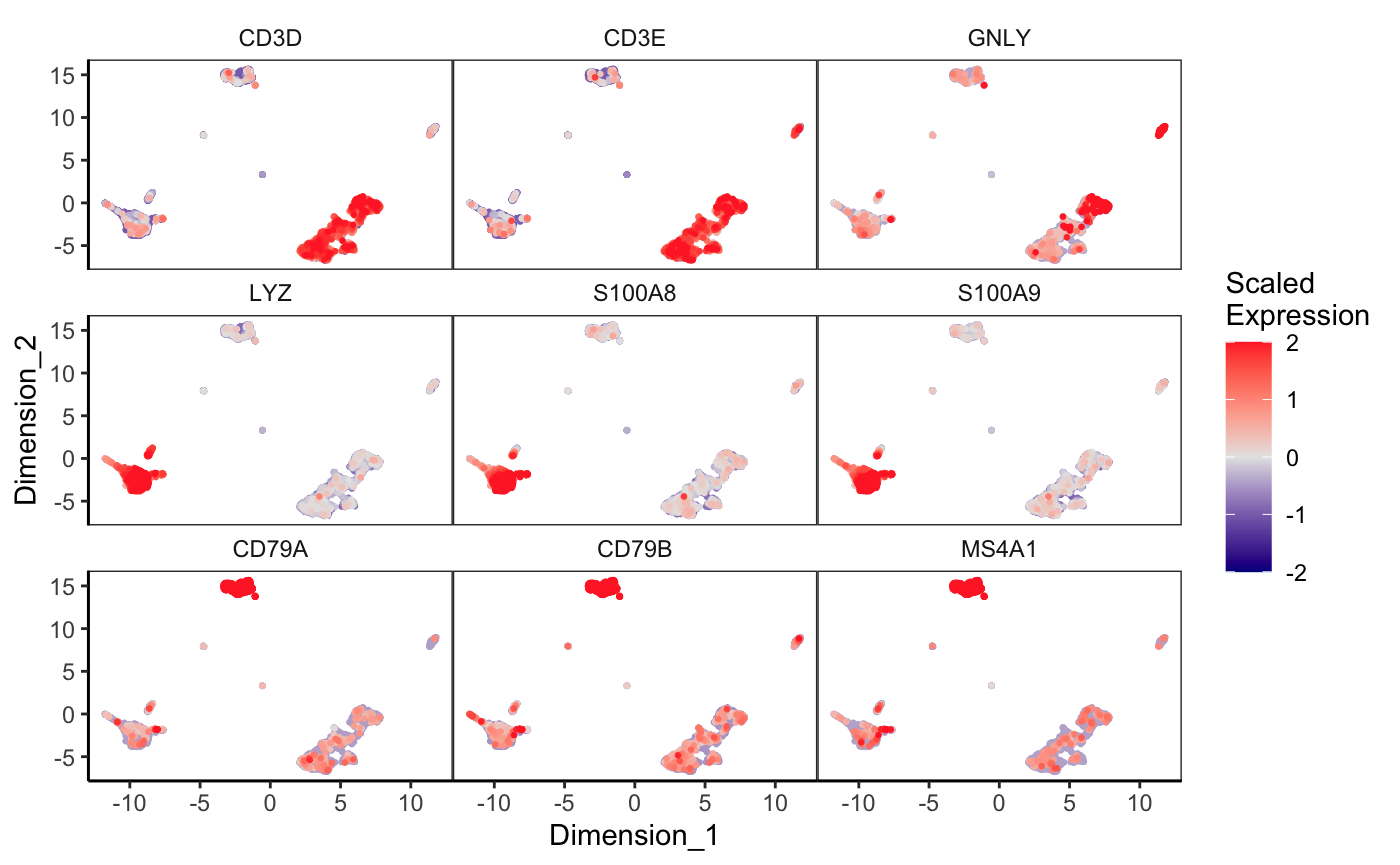
Barplot of markers detected in cell clusters
The percetage of cells within a cluster that have detectable expression of marker genes can be displayed in a barplot. Markers for cell types need to be supplied in a named list. First, the detection of marker genes in the original counts assay is shown:
markers <- list(Tcell_Markers = c("CD3E", "CD3D"),
    Bcell_Markers = c("CD79A", "CD79B", "MS4A1"),
    Monocyte_Markers = c("S100A8", "S100A9", "LYZ"),
    NKcell_Markers = "GNLY")
cellTypeMappings <- list(Tcells = 2, Bcells = 5, Monocytes = 1, NKcells = 6)
plotDecontXMarkerPercentage(sce,
    markers = markers,
    groupClusters = cellTypeMappings,
    assayName = "counts")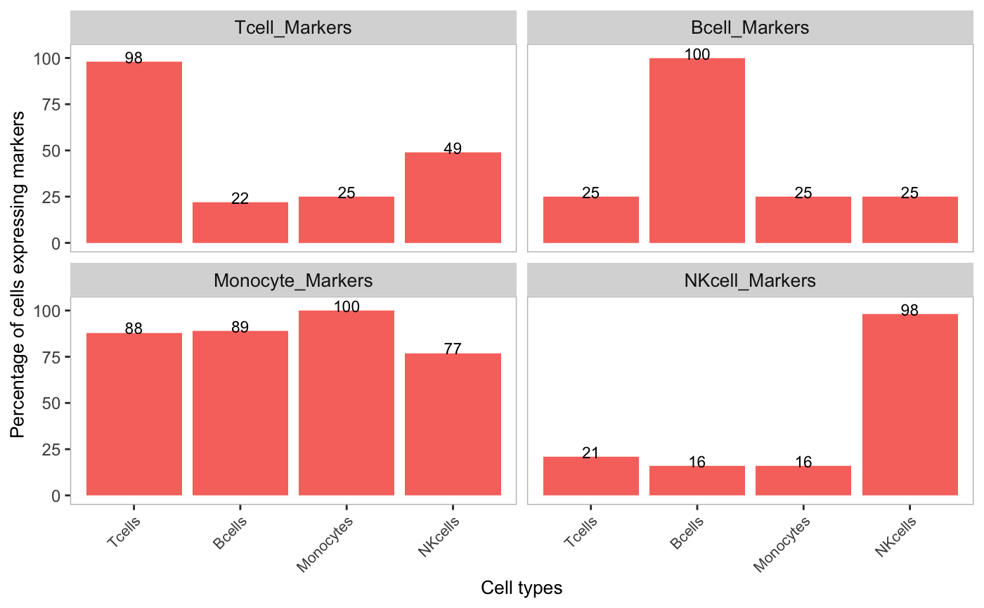
We can then look to see how much decontX removed aberrant expression of marker genes in each cell type by changing the assayName to decontXcounts:
plotDecontXMarkerPercentage(sce,
    markers = markers,
    groupClusters = cellTypeMappings,
    assayName = "decontXcounts")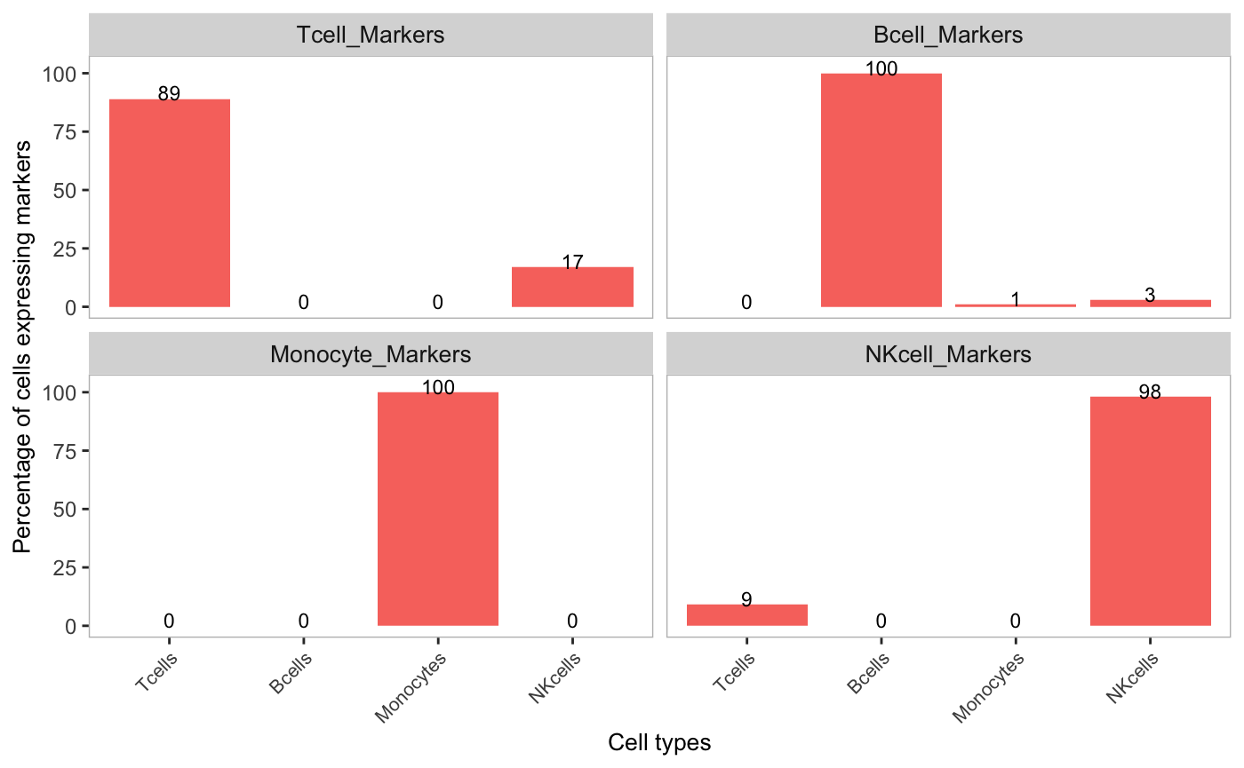
Percentages of marker genes detected in other cell types were reduced or completely removed. For example, the percentage of cells that expressed Monocyte marker genes was greatly reduced in T-cells, B-cells, and NK-cells. The original counts and decontamined counts can be plotted side-by-side by listing multiple assays in the assayName parameter. This option is only available if the data is stored in SingleCellExperiment object.
plotDecontXMarkerPercentage(sce,
    markers = markers,
    groupClusters = cellTypeMappings,
    assayName = c("counts", "decontXcounts"))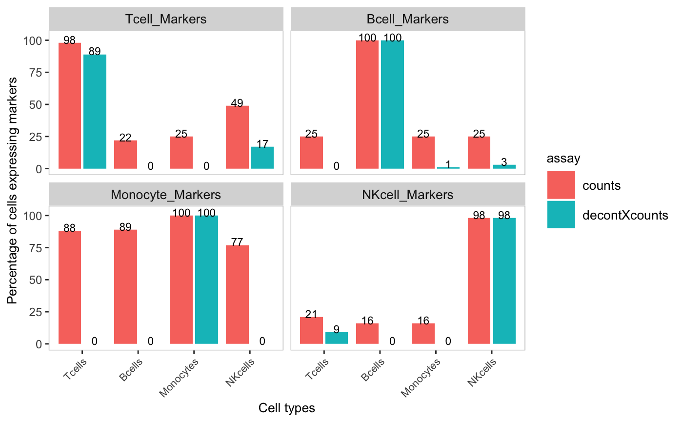
Some helpful hints when using plotDecontXMarkerPercentage:
- Cell clusters can be renamed and re-grouped using the
groupClusterparameter, which also needs to be a named list. IfgroupClusteris used, cell clusters not included in the list will be excluded in the barplot. For example, if we wanted to group T-cells and NK-cells together, we could setcellTypeMappings <- list(NK_Tcells = c(2,6), Bcells = 5, Monocytes = 1) - The level a gene needs to be expressed to be considered detected in a cell can be adjusted using the
thresholdparameter. - If you are not using a
SingleCellExperiment, then you will need to supply the original counts matrix or the decontaminated counts matrix as the first argument to generate the barplots.
Violin plot to compare the distributions of original and decontaminated counts
Another useful way to assess the amount of decontamination is to view the expression of marker genes before and after decontX across cell types. Here we view the monocyte markers in each cell type. The violin plot shows that the markers have been removed from T-cells, B-cells, and NK-cells, but are largely unaffected in monocytes.
plotDecontXMarkerExpression(sce,
    markers = markers[["Monocyte_Markers"]],
    groupClusters = cellTypeMappings,
    ncol = 3)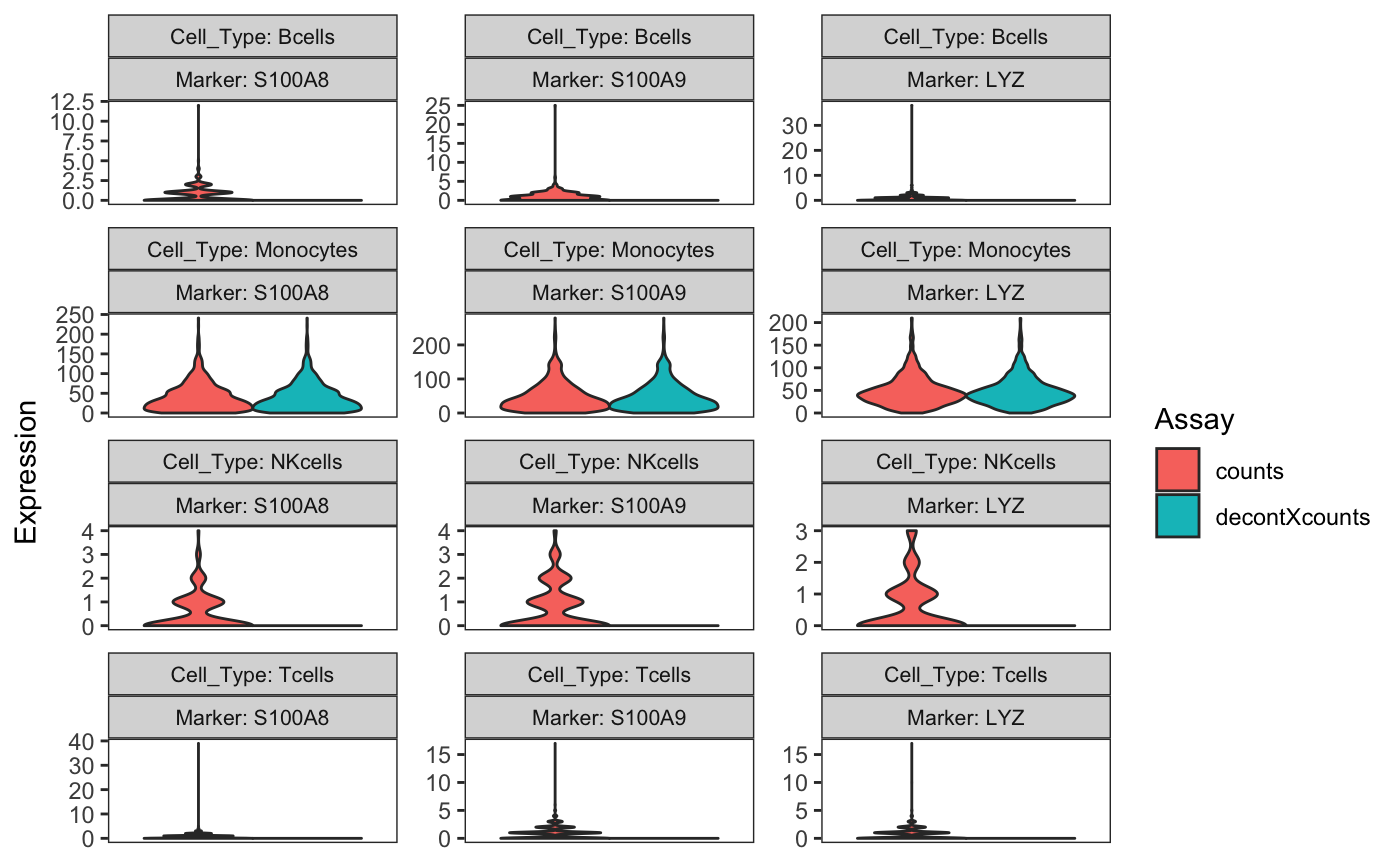
Some helpful hints when using plotDecontXMarkerExpression:
-
groupClustersworks the same way as inplotDecontXMarkerPercentage. - This function will plot each pair of markers and clusters (or cell type specified by
groupClusters). Therefore, you may want to keep the number of markers small in each plot and call the function multiple times for different sets of marker genes. - You can also plot the individual points by setting
plotDots = TRUEand/or log transform the points on the fly by settinglog1p = TRUE. - This function can plot any assay in a
SingleCellExperiment. Therefore you could also examine normalized expression of the original and decontaminated counts. For example:
sce <- scater::logNormCounts(sce,
    exprs_values = "decontXcounts",
    name = "dlogcounts")

plotDecontXMarkerExpression(sce,
    markers = markers[["Monocyte_Markers"]],
    groupClusters = cellTypeMappings,
    ncol = 3,
    assayName = c("logcounts", "dlogcounts"))
Other important notes
Choosing appropriate cell clusters
The ability of DecontX to accurately identify contamination is dependent on the cell cluster labels. DecontX assumes that contamination for a cell cluster comes from combination of counts from all other clusters. The default clustering approach used by DecontX tends to select fewer clusters that represent broader cell types. For example, all T-cells tend to be clustered together rather than splitting naive and cytotoxic T-cells into separate clusters. Custom cell type labels can be suppled via the z parameter if some cells are not being clustered appropriately by the default method.
Adjusting the priors to influence contamination estimates
There are ways to force decontX to estimate more or less contamination across a dataset by manipulating the priors. The delta parameter is a numeric vector of length two. It is the concentration parameter for the Dirichlet distribution which serves as the prior for the proportions of native and contamination counts in each cell. The first element is the prior for the proportion of native counts while the second element is the prior for the proportion of contamination counts. These essentially act as pseudocounts for the native and contamination in each cell. If estimateDelta = TRUE, delta is only used to produce a random sample of proportions for an initial value of contamination in each cell. Then delta is updated in each iteration. If estimateDelta = FALSE, then delta is fixed with these values for the entire inference procedure. Fixing delta and setting a high number in the second element will force decontX to be more aggressive and estimate higher levels of contamination in each cell at the expense of potentially removing native expression. For example, in the previous PBMC example, we can see what the estimated delta was by looking in the estimates:
metadata(sce)$decontX$estimates$all_cells$delta## [1] 9.287164 1.038217Setting a higher value in the second element of delta and estimateDelta = FALSE will force decontX to estimate higher levels of contamination per cell:
sce.delta <- decontX(sce, delta = c(9, 20), estimateDelta = FALSE)

plot(sce$decontX_contamination, sce.delta$decontX_contamination,
     xlab = "DecontX estimated priors",
     ylab = "Setting priors to estimate higher contamination")
abline(0, 1, col = "red", lwd = 2)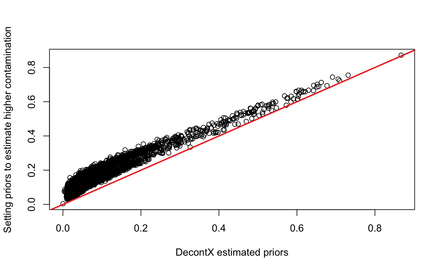
Session Information
## R version 4.0.4 (2021-02-15)
## Platform: x86_64-apple-darwin17.0 (64-bit)
## Running under: macOS Big Sur 10.16
##
## Matrix products: default
## BLAS:   /Library/Frameworks/R.framework/Versions/4.0/Resources/lib/libRblas.dylib
## LAPACK: /Library/Frameworks/R.framework/Versions/4.0/Resources/lib/libRlapack.dylib
##
## locale:
## [1] en_US.UTF-8/en_US.UTF-8/en_US.UTF-8/C/en_US.UTF-8/en_US.UTF-8
##
## attached base packages:
## [1] parallel  stats4    stats     graphics  grDevices utils     datasets
## [8] methods   base
##
## other attached packages:
##  [1] scater_1.18.6               ggplot2_3.3.5
##  [3] TENxPBMCData_1.8.0          HDF5Array_1.18.1
##  [5] rhdf5_2.34.0                DelayedArray_0.16.2
##  [7] Matrix_1.3-2                SingleCellExperiment_1.12.0
##  [9] SummarizedExperiment_1.20.0 Biobase_2.50.0
## [11] GenomicRanges_1.42.0        GenomeInfoDb_1.26.4
## [13] IRanges_2.24.1              S4Vectors_0.28.1
## [15] BiocGenerics_0.36.0         MatrixGenerics_1.2.1
## [17] matrixStats_0.58.0          celda_1.9.2
##
## loaded via a namespace (and not attached):
##   [1] AnnotationHub_2.22.0          BiocFileCache_1.14.0
##   [3] systemfonts_1.0.1             RcppEigen_0.3.3.9.1
##   [5] plyr_1.8.6                    assertive.files_0.0-2
##   [7] enrichR_3.0                   multipanelfigure_2.1.2
##   [9] BiocParallel_1.24.1           digest_0.6.27
##  [11] foreach_1.5.1                 htmltools_0.5.1.1
##  [13] viridis_0.5.1                 magick_2.7.0
##  [15] fansi_0.4.2                   magrittr_2.0.1
##  [17] memoise_2.0.0                 assertive.numbers_0.0-2
##  [19] doParallel_1.0.16             pkgdown_1.6.1
##  [21] colorspace_2.0-0              blob_1.2.1
##  [23] rappdirs_0.3.3                ggrepel_0.9.1
##  [25] textshaping_0.3.5             xfun_0.22
##  [27] dplyr_1.0.5                   crayon_1.4.1
##  [29] RCurl_1.98-1.2                jsonlite_1.7.2
##  [31] iterators_1.0.13              glue_1.4.2
##  [33] gtable_0.3.0                  zlibbioc_1.36.0
##  [35] XVector_0.30.0                BiocSingular_1.6.0
##  [37] Rhdf5lib_1.12.1               scales_1.1.1
##  [39] DBI_1.1.1                     Rcpp_1.0.6
##  [41] viridisLite_0.3.0             xtable_1.8-4
##  [43] gridGraphics_0.5-1            bit_4.0.4
##  [45] rsvd_1.0.3                    httr_1.4.2
##  [47] RColorBrewer_1.1-2            ellipsis_0.3.1
##  [49] farver_2.1.0                  pkgconfig_2.0.3
##  [51] scuttle_1.0.4                 sass_0.3.1
##  [53] uwot_0.1.10                   dbplyr_2.1.0
##  [55] utf8_1.2.1                    labeling_0.4.2
##  [57] tidyselect_1.1.0              rlang_0.4.10
##  [59] reshape2_1.4.4                later_1.1.0.1
##  [61] AnnotationDbi_1.52.0          munsell_0.5.0
##  [63] BiocVersion_3.12.0            tools_4.0.4
##  [65] cachem_1.0.4                  dbscan_1.1-6
##  [67] generics_0.1.0                RSQLite_2.2.4
##  [69] ExperimentHub_1.16.0          evaluate_0.14
##  [71] stringr_1.4.0                 fastmap_1.1.0
##  [73] yaml_2.2.1                    ragg_1.1.3
##  [75] knitr_1.31                    bit64_4.0.5
##  [77] fs_1.5.0                      purrr_0.3.4
##  [79] sparseMatrixStats_1.2.1       mime_0.10
##  [81] compiler_4.0.4                beeswarm_0.3.1
##  [83] curl_4.3                      interactiveDisplayBase_1.28.0
##  [85] tibble_3.1.0                  bslib_0.2.4
##  [87] stringi_1.5.3                 highr_0.8
##  [89] desc_1.3.0                    RSpectra_0.16-0
##  [91] lattice_0.20-41               assertive.base_0.0-9
##  [93] vctrs_0.3.6                   pillar_1.5.1
##  [95] lifecycle_1.0.0               rhdf5filters_1.2.0
##  [97] BiocManager_1.30.10           combinat_0.0-8
##  [99] jquerylib_0.1.3               RcppAnnoy_0.0.18
## [101] BiocNeighbors_1.8.2           data.table_1.14.0
## [103] bitops_1.0-6                  irlba_2.3.3
## [105] httpuv_1.5.5                  assertive.types_0.0-3
## [107] R6_2.5.0                      assertive.properties_0.0-4
## [109] promises_1.2.0.1              gridExtra_2.3
## [111] vipor_0.4.5                   codetools_0.2-18
## [113] MCMCprecision_0.4.0           assertthat_0.2.1
## [115] rprojroot_2.0.2               rjson_0.2.20
## [117] withr_2.4.1                   GenomeInfoDbData_1.2.4
## [119] grid_4.0.4                    beachmat_2.6.4
## [121] rmarkdown_2.7                 DelayedMatrixStats_1.12.3
## [123] Rtsne_0.15                    shiny_1.6.0
## [125] ggbeeswarm_0.6.0